
Fizeau experiment path-length convention 2026-10-18
Use the schematic below to count the water traversals explicitly. Each stationary tube has laboratory length . In the displayed setting, upper-tube water flows right and lower-tube water flows left, each at speed . Beam A goes right through the upper tube, exchanges tubes at the far optics, and returns left through the lower tube: it follows the flow twice. Beam B goes right through the lower tube and returns left through the upper tube: it opposes the flow twice. Each complete beam path therefore contains total water length , not or . The connecting air paths and fixed optics are assumed to contribute no flow-dependent phase difference.
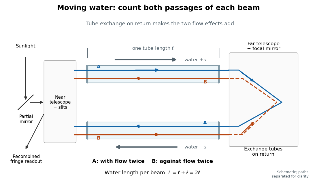
Counterflow path accounting: beam A follows the water in both tubes, beam B opposes it, and each beam traverses total water length 2ℓ
. Original schematic of the tube exchange and recombination, not a scaled optical ray trace. Parallel coloured lines separate overlapping counterpropagating beams for readability. The grey arrows show water flow; reversing both grey arrows exchanges the roles of A and B. Details.
Let and be positive phase velocity magnitudes along and against the water flow:For a laboratory source of frequency , where is its vacuum wavelength, define the signed interference fringe offset by the propagation phase difference . This is an equivalent phase delay between steady beams; no stopwatch resolves their transit-time difference. Subtract the zero-flow baseline and expand to first order:Thus one shifted fringe corresponds to one cycle of phase difference. If the stationary pattern has spatial interference fringe spacing , a simple readout model is , where is the interference visibility. The maxima shift by with this choice of screen coordinate. A sign assigned to “rightward” motion depends on the image orientation; the magnitude in fringe units does not.
Reversing both flows gives . The displacement between equal and opposite settings therefore has magnitudeThe factor from comparing opposite flows is additional to the factor already included in . Repeating a round trip in just one flowing tube would instead put a beam with the flow once and against it once; that geometry does not produce the two same-sign contributions drawn here.
Fresnel drag coefficient Created 2026-10-18 Updated 2026-10-25
The Fresnel drag coefficient is the factor multiplying a transparent medium's velocity in the first-order change of collinear light phase velocity, when optical dispersion is neglected. Here is the medium's refractive index in its rest frame. The name recalls Augustin-Jean Fresnel's partial-drag law; special relativity obtains the same coefficient from the velocity-addition formula without introducing a luminiferous aether.
Let the water move at signed velocity along the positive laboratory axis, with , where is the vacuum speed of light. Assume a transparent medium with constant , uniform flow and negligible optical dispersion. In the water's local rest frame, a collinear constant-phase surface travels at . Dividing the Lorentz transformation differentials along that surface gives the same longitudinal velocity-addition formula as for a particle:The correction comes from the transformed time denominator. Simply adding to would omit it. This argument concerns collinear phase velocity; in a medium with optical dispersion, group velocity is a different quantity.[ref]
Fizeau’s “Aether-Drag” Experiment in the Undergraduate Laboratory by Thierry Lahaye and others. Section III, pp. 498–499, equation (1) and discussion of the collinear wave-four-vector derivation
For , the Fresnel drag coefficient is . A chosen flow speed of therefore changes the forward phase velocity by approximately , even though the stationary-medium phase velocity is about . These are model values. The invariant vacuum speed of light remains ; describes propagation through matter in its own rest frame.
Dielectric insertion force at fixed voltage 2026-10-18
At fixed electric potential difference , a change of capacitance has electrical work input and field-energy increase . The remaining half is mechanical work done by the field, so the force in the direction of increasing overlap is . Equivalently the effective mechanical potential is . For a partially filled coaxial capacitor, this gives , directed inward when . The fringing field of a capacitor supplies the local field gradient and transmits this force even when its small correction to total capacitance is neglected.
Optimal fixed step for quadratic gradient descent Created 2026-10-18 Updated 2026-10-31
For a fixed symmetric matrix and positive-definite matrix , what positive step size minimizes the largest coordinate error multiplier over all eigenvector directions? Let and . Since is a convex function of , its maximum over the eigenvalues occurs at an endpoint:Balance the two extremes by solving :Here is the Euclidean norm condition number of . This balance is optimal: for the endpoint exceeds , and for the endpoint exceeds . The optimal worst-case energy factor is , rather than . This optimizes a uniform one-step bound; a particular initial error supported on fewer eigenvectors can have a different best step size.
In the example , , so and . Both eigenvalue directions attain that energy factor, making the displayed history exact. The smaller step size instead givesIts first step reaches , below for , but subsequent progress is limited by the first direction's energy factor . By , the energies are approximately and , respectively; by , the iteration is ahead. A better first step need not yield a faster long-run history.
As the condition number grows, approaches one: stability in the direction of the largest eigenvalue forces small movement along the smallest-eigenvalue direction. This is a precise reason to improve scaling or use a method such as the conjugate gradient method, rather than merely increasing the step size. When , choosing eliminates every error component in one step.
Polarization overlap in interferometric visibility Created 2026-10-18 Updated 2026-11-05
For perfectly temporally coherent beams with unit Jones vectors , their interference term is proportional to the complex inner product . Their interferometric visibility is the displayed expression. Equal beam light intensities reduce it to the magnitude of the polarization overlap. Two linear polarizations at relative angle give ; a linear and a circular polarization give . Perfect coherence does not remove loss of contrast from unequal intensities or orthogonal polarizations.
Etalon resolving power and order overlap 2026-10-18
For an ideal air-gap Fabry–Pérot etalon at normal incidence, the free spectral range is and the peak full width at half maximum is . To separate a pair of lines spaced by by at least peak widths, require . Putting both lines inside one unambiguous free spectral range additionally requires , so . In terms of their vacuum wavelengths, .
The strict order condition needs a margin if tails from adjacent periodic peaks are to be negligible. If every neighbouring peak in a scanned two-line periodic spectrum must be separated by widths, the stronger condition is . Ordinary resolving power alone does not prevent ambiguous repeated orders. A fixed etalon's transmission as a function of wavelength is a periodic-in-frequency filter; it is not automatically a plot of the incident source's spectral lines.
Fibonacci recurrence 2026-10-18
The linear recurrence relation defining the Fibonacci numbers, with and . Its state advances by the matrix , so matrix powers describe repeated updates.
Barkhausen effect Created 2026-10-18 Updated 2026-10-20
The Barkhausen effect consists of abrupt magnetization changes during a smooth applied magnetic field sweep. Its inductive signal is Barkhausen noise, often arising from collective magnetic domain wall motion.[ref]
The distinction is between a smooth drive and an intermittent material response. A smooth macroscopic hysteresis curve can hide smaller jumps. By Faraday's law of induction, a pickup coil responds to the rate of change of linked magnetic flux, so a rapid jump can be conspicuous even when the total change is small. A pulse is not one chemical atom flipping: neither its height nor the number of audible clicks counts individual electron spins. Qualitative crackling alone does not establish quantum spin; collective switching also admits a classical model with trapped interfaces. Compare the distinct mechanical readout of angular momentum transfer in the Einstein-de Haas effect.
Magnetic domain 2026-10-18
A magnetic domain is a region sharing an ordered magnetic orientation. Different magnetic domains can reduce the total magnetic moment without erasing the local magnetic order. A zero total magnetization therefore does not by itself establish antiferromagnetism.
Ferromagnet Created 2026-10-18 Updated 2026-10-20
A ferromagnet is a material that exhibits ferromagnetism. Its magnetic domains can cancel the net magnetization even while each domain remains ordered.
Two-dimensional electron gas Created 2026-10-18 Updated 2026-10-20
An electron gas confined in one spatial direction, with motion available in the other two. Its electron number per unit area is . The ideal Fermi gas approximation neglects interactions between electrons; an actual two-dimensional electron gas can have important interactions. Confinement alone does not require a magnetic field or Landau levels.
Coupled RL induction model 2026-10-18
Take two electrical circuits containing coupled inductors. Let their constant self-inductances be , mutual inductance , and positive electrical resistances . Choose current directions so that the off-diagonal entries of the inductance matrix are . Assume a linear, quasistatic model, with no capacitive effects or core hysteresis. The magnetic flux linkages are and . Combining their time derivatives with resistive electric potential differences givesThe secondary is a closed, undriven electrical circuit. Require , making a positive-definite matrix. The chosen current convention fixes the signs; reversing the secondary's reference direction changes the sign assigned to and without changing the physical circuit.
There is an essential switching assumption: the primary loop remains closed when becomes zero. An ideal voltage source then imposes zero electric potential difference, allowing the current to decay. Literally opening an inductive circuit requires additional physics to determine the interruption, including possible capacitance and an electric arc. This closed-return model explains transient induction while keeping that distinction from Faraday's historical making and breaking of contact explicit.
COBE FIRAS blackbody spectrum experiment 2026-10-18
FIRAS compared sky radiation with an adjustable internal blackbody using an interferometer and cold bolometers. An external blackbody could cover the sky entrance for measurement calibration. The team adjusted the internal temperature to minimize the difference signal.[ref]
Nobel Lecture: From the Big Bang to the Nobel Prize and beyond by John C. Mather. §III.D, pp.1337–1338; §V.A, p.1341
Comparisons across detectors and mirror strokes tested instrumental errors; sky mapping separated Milky Way emission. John C. Mather's lecture reports a final root-mean-square spectral departure of 50 parts per million of peak brightness. This is neither the preliminary 1990 precision nor a relative error in every spectral bin. Calibration drift and nonideal reference emission required correction.[ref]
Nobel Lecture: From the Big Bang to the Nobel Prize and beyond by John C. Mather. §V.A, p.1342: calibration checks and final spectrum
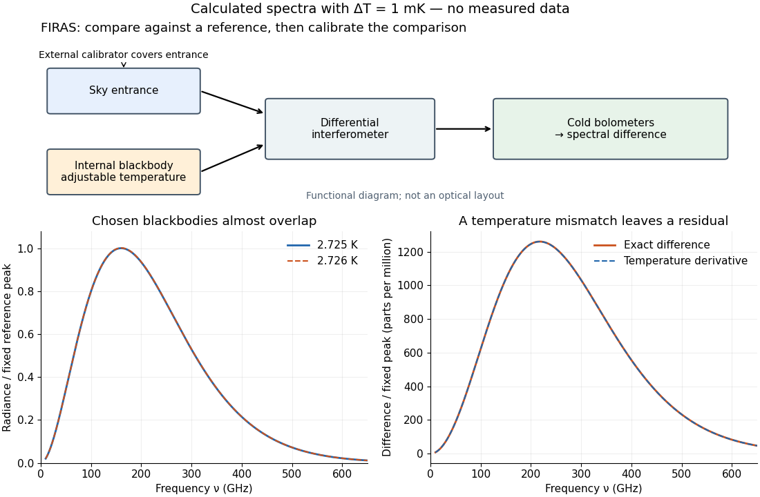

The advantage of a null measurement is that a small difference can be resolved without assigning the same absolute precision to a large detector output. Nevertheless, matching an internal reference is meaningful only after its relation to an independently calibrated blackbody has been tested. A bound on departures from a Planck spectrum constrains energy redistribution after thermal equilibrium; it does not require the cosmic microwave background to have exactly the same temperature in every direction.
For the formal one-dimensional operator with and , take a smooth normalized test function supported away from the origin. Its normalized dilation hasAs , this tends to minus infinity. Thus the unregularized expression has fall to the centre for a supercritical inverse-power potential and cannot define a semibounded Hamiltonian operator on a domain containing these test functions.
If a putative bound state has separately finite and admits norm-preserving dilation variations inside its operator domain or energy domain, stationarity gives , hence , incompatible with a negative-energy bound state below the zero continuum threshold. For a putative ground state, the second scaling derivative is , also incompatible with a minimum. The argument's finite-energy and domain assumptions are essential: it proves absence of a stable ground state and excludes bound states to which this ordinary virial calculation applies. An unqualified assertion about all formal square-integrable solutions at the singular origin needs a specified self-adjoint realization; adding a short-distance cutoff changes the problem.
Faithful quotient of a group action 2026-10-18
For any group action with group kernel , the quotient group has a faithful group action on the same set, given byTo check independence of the coset representative, replace by with : then . If fixes every point, then , so , the identity element of the quotient group. The first isomorphism theorem identifies this quotient group with the image of inside the symmetric group. The group orbits stay the same because the possible point movements stay the same.
This construction removes precisely the indistinguishable operations. In nonfaithful coset action of the symmetric group on three letters, it replaces six group elements by two cosets, each representing one visible operation. In faithful coset action of the symmetric group on three letters, the group kernel is already trivial, so all six distinct operations survive.
Let , the symmetric group on three letters, and take the normal subgroup , the alternating group of even permutations. Its two left cosets areProducts of permutations apply the rightmost factor first. Left multiplication by an even permutation preserves both cosets, while left multiplication by an odd permutation exchanges them. For example,Consequently all six group elements give only two distinct permutations of . Both stabilizer subgroups equal , so their intersection, the group kernel, is . This is a transitive group action because reaches the other coset, but it is not a faithful group action because fixes both.
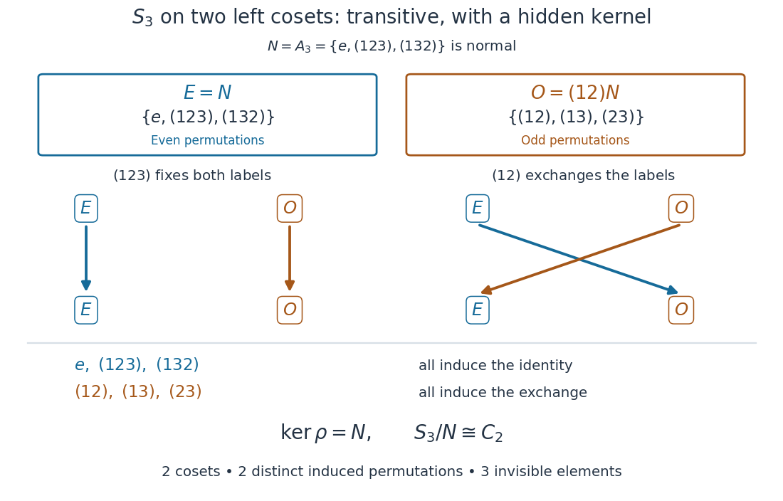

The orbit-stabilizer theorem still works perfectly: . It counts reachable labels, without asserting that the induced group homomorphism is injective. The quotient group captures exactly the two visible operations, identity and exchange. This is the same group homomorphism as the sign of a permutation, with represented by fixing both labels and by exchanging them. Contrast the three-label example in faithful coset action of the symmetric group on three letters.
After integrating out other variables, let include the constrained entropy and the measure appropriate to the chosen coordinate . Its equilibrium probability density function is proportional to . Near a stable interior minimum, with . The resulting normal distribution has variance . This is the leading Gaussian fluctuation approximation; a coordinate-dependent measure contributes to the effective , and higher-order terms matter near a vanishing curvature.
Excluded-volume ideal gas 2026-10-18
For one mole, a simple repulsive-volume model uses with and domain . The Maxwell relation and first law of thermodynamics give , so . If its molar heat capacity at constant volume is temperature independent, it is constant, and . Reversible adiabatic processes obey or . All positive-temperature isotherms are strictly decreasing and convex; this single-phase model contains no attractive liquid-gas coexistence mechanism. The parameter is an effective unavailable molar volume, not automatically the literal geometric volume of the molecules.
Let be a twice continuously differentiable function on an open domain stable under positive scaling, with . Apply the chain rule twice to the scalar function and set . The result isIn two variables, this reads . In matrix notation it is , where is the Hessian matrix. Equivalently, the radial differential operator obeys ; substituting explains the factor .
For a twice continuously differentiable homogeneous function of degree one, Euler theorem for homogeneous functions gives . Differentiation first with respect to and then, separately, with respect to givesMultiplying by and , respectively, shows that . This identity can verify a second-order partial differential equation without expanding a complicated homogeneous expression twice.
There are unlisted articles, also show them or only show them.