
Positive compression contributes negative quadratic potential energy , while positive bending stiffness contributes . A plane wave has , so sufficiently long waves grow exponentially. For displacement-fixed, moment-free endpoints at , the natural boundary conditions for a free endpoint on the slope give as well as . The modes are , and the first Euler buckling of an elastic filament threshold is . For truly clamped ends, , the threshold is instead , with first static mode . More generally,with the infimum taken over the specified endpoint class. At threshold there is a static zero mode and a marginal linear-in-time partner in the linear dynamics; above it the straight configuration is unstable.
Euler's critical load 2026-10-18
A straight slender elastic beam under axial compression loses stability when bending can decrease its total potential energy. With pinned ends a distance apart, its quadratic potential is . Stationarity gives , with at each end. The first nontrivial mode is , at . More generally , with an effective-length factor determined by endpoint constraints: for pinned-pinned, for fixed-free and for fixed-fixed. Real imperfections remove the perfectly sharp onset, and short columns can yield before this elastic instability.
Clamped-beam Green function Created 2026-10-18 Updated 2026-11-05
For a unit-length elastic beam with unit bending stiffness, the Green function of with at both endpoints is the displayed kernel. It is piecewise cubic and continuous through its second derivative, while . A constructive form is , with and . The right endpoint conditions determine these coefficients. Thus solves the clamped static beam problem.
Distance from a point to a line Created 2026-10-18 Updated 2026-10-31
For a line with , its unit normal is . Choose any point on the line and project the displacement to onto this normal. The absolute value of that projection gives the title formula. This is the shortest Euclidean distance, because any displacement to a different point on the line has the same normal component and an additional orthogonal tangential component.
Compressibility factor 2026-10-18
The compressibility factor is the ratio , where is number density. A classical ideal gas has . The virial expansion writes for a dilute gas; this dimensionless ratio is distinct from isothermal compressibility, which is a response derivative with units of inverse pressure.
Shubnikov-de Haas effect Created 2026-10-18 Updated 2026-11-05
The Shubnikov-de Haas effect is an oscillatory variation of electrical resistance with magnetic field caused by Landau levels moving through the Fermi energy. As the density of accessible states near that energy changes, the conductivity and scattering response oscillate.
A measurement sweeps field at low temperature while recording a longitudinal voltage for a controlled current. Oscillations are commonly approximately periodic in inverse field for a fixed closed Fermi-surface orbit. Their period probes the orbit area, while temperature-dependent amplitude constrains a cyclotron effective mass. Disorder and thermal broadening can wash out the oscillations even when a Fermi surface exists. The effect is a transport measurement, distinct from the oscillating magnetization measured in the thermodynamic quantum-oscillation counterpart.
Cyclotron effective mass 2026-10-18
For a closed semiclassical orbit with area in a plane of wave vector space, the cyclotron effective mass is defined by the displayed derivative. It need not equal the local curvature-based band effective mass.
Electronic valley 2026-10-18
A region of wave vector space around a low-energy band feature, such as a band minimum or a Dirac point.
Dirac cone 2026-10-18
A conical touching of two energy bands, with locally linear dispersion relation. The nearest-neighbour model of graphene supplies an explicit example.
Electronic bandwidth Created 2026-10-18 Updated 2026-10-20
The electronic bandwidth is the difference between the maximum and minimum of one energy band over the Brillouin zone. It has units of energy, unlike a frequency bandwidth in signal processing. A nearest-neighbour tight-binding model on a primitive cubic lattice with equal real hopping integrals has and .
Complete elliptic integral of the second kind Created 2026-10-18 Updated 2026-10-20
For , define . An ellipse with semi-major and semi-minor axes and eccentricity of a conic has perimeter . Differentiating its parametrization gives the speed , and fourfold symmetry reduces the full arc length to a quadrant. The binomial series gives near zero.
Degree drop in a specialized resultant 2026-10-18
The actual-degree condition in the resultant theorem matters when coefficients depend on a parameter. TakeThe nominal degree-one Sylvester matrix is , whose determinant is . Its specialization at therefore vanishes. But the specialized polynomials are the nonzero constants and , which have no common root at all.
For , the roots of a polynomial are and ; neither has a finite limit as . Both leading coefficients vanish at the exceptional parameter. The fixed-size determinant has retained the original degree format even though the specialized polynomial degrees have dropped. Recompute using the actual specialized polynomials and check the original equations before accepting a zero of a parameter-dependent resultant as a solution.
Trapped-ion fluorescence count model 2026-10-18
For an original illustrative readout model, take detected photon count in a fixed exposure to have a Poisson distribution, with stipulated means for a bright state and for a dark state. Classify as bright. Direct summation givesWith equally likely preparations, the average misclassification probability is . These numbers describe only the chosen count model. Actual fluorescence includes short-time photon correlations, detector effects and possible state changes; it need not follow a fixed-rate Poisson process. Longer exposure can improve separation of count distributions while increasing unwanted optical pumping, metastable decay or recoil.
If the prepared bright population is , let and denote the two conditional errors above. The observed bright-label probability is , hence when the denominator is nonzero. Known-state controls must estimate in the actual apparatus; the formula cannot correct unknown drift. For independent preparations, the raw bright fraction has variance . Counting uncertainty, preparation error, pulse error and state-detection bias therefore enter different parts of the inference. Repeating a biased measurement reduces its sampling uncertainty without removing its bias.
Transmission electron microscopy Created 2026-10-18 Updated 2026-10-20
Transmission electron microscopy images electrons transmitted through a thin specimen. Electron diffraction from a selected region supplies complementary information about its atomic arrangement. A useful transmitted signal requires suitable specimen thickness.[ref]
Transmission Electron Microscope (TEM) by JEOL. JEOL, Another characteristic electron diffraction: thin specimens, images and diffraction patterns
The image also depends on which outgoing electron directions reach the detector. Transmission electron microscopy contrast makes this selection explicit: changing the objective aperture can change an image without changing the specimen. Interpreting the result requires electron diffraction, a specified detector response and measurement calibration.
Spin-orbit g-factor ratio from two P states 2026-10-18
An original reduced model makes the cancellation explicit. Assume LS coupling, neglect nuclear spin, and write the electronic magnetic dipole moment as . For , , the projection used to derive the Landé g-factor givesThese coefficients follow by substituting or into the angular-momentum projection formula; neither level measures pure spin alone. In a weak uniform magnetic field, adjacent electronic projections have spacing when . ThereforeThe common magnetic field and Bohr magneton cancel. The ratio determines , not without further knowledge of . For , it gives . Small departures from are magnified differently from small departures of from ; the two fractional changes should not be identified.
With the stipulated inputs , and , the two electronic frequencies are and . Their ratio is approximately , and inversion recovers . These are ideal electronic lines, not historical gallium data. Nuclear spin, mixing between levels and other deviations from LS coupling require a more complete model in an actual atom.
Kusch-Foley magnetic moment experiment 2026-10-18
Polykarp Kusch and Henry Michael Foley compared hyperfine structure resonance frequencies for different electronic states of gallium, indium and sodium. Their 1948 paper reports mutually consistent departures from the ratios expected with orbital factor and spin factor . Comparing several states constrained the alternative explanation of perturbed atomic levels.[ref]
The Magnetic Moment of the Electron by Polykarp Kusch and Henry Michael Foley (1948). Abstract: atomic states, frequency comparisons and interpretation
The Rabi molecular beam magnetic resonance experiment explains the readout principle: a resonant transition changes an atom's magnetic response, and hence its transmitted beam signal. Kusch describes rapidly interchangeable ovens, several radio frequency oscillators and careful field homogenization. Measurements taken during monotonic field drift were reduced to a common field.[ref]
The magnetic moment of the electron by Polykarp Kusch. pp. 303–304: resonance analysis, ovens, oscillators and field drift
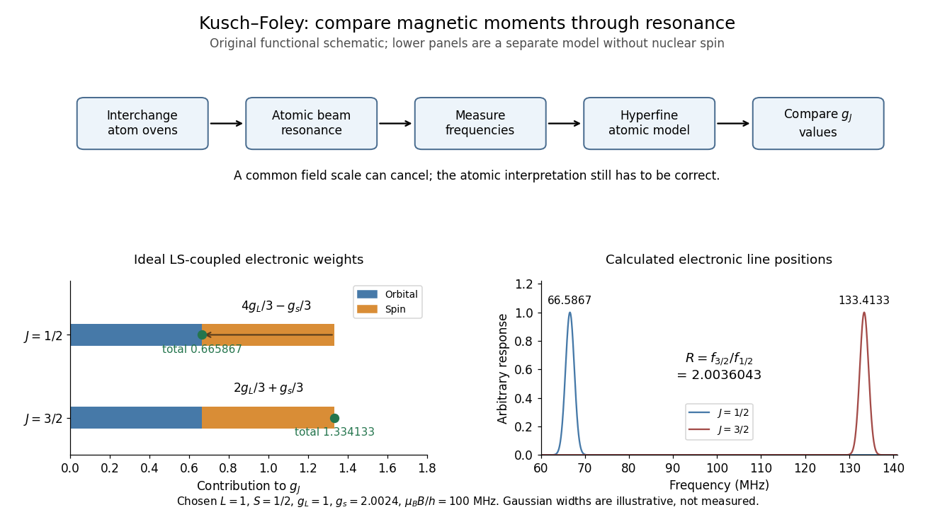
Compare differently weighted atomic magnetic moments
. Original functional diagram of the Kusch-Foley magnetic moment experiment and a separate ideal LS coupling calculation. The upper flow identifies the functions of beam preparation, resonance readout and atomic modeling; it is not a surviving apparatus drawing. The lower weights are calculated for , , and chosen , without nuclear spin. The frequencies in the teaching model cannot be substituted directly for measured hyperfine lines. Details.
Real hyperfine structure lines are not simply bare electronic times field. Nuclear magnetic moments, known interaction constants and nonlinear field dependence enter the inference.[ref]
The magnetic moment of the electron by Polykarp Kusch. pp. 303–305: hyperfine modeling and atomic-state perturbations
Field homogeneity controls line broadening; alternating species addresses drift. Neither control removes an error in the atomic model. The beauty of the comparison is the separation of two problems: cancelling a shared calibration scale and testing whether several physical systems imply the same electron spin g-factor. Electron spin g-factor 2026-10-18
The dimensionless coefficient in the spin part of the electron magnetic moment. It is distinct from a gyromagnetic ratio, which has units: in the angular convention, . It is also distinct from the Landé g-factor of a combined atomic angular momentum and from a nuclear or hyperfine g-factor.
For spin one-half, the largest magnitude of a spin-component magnetic dipole moment is , not . Thus the ideal value gives one Bohr magneton. This follows directly from the spin angular momentum projections .
Choose coordinates and Minkowski metric . With the convention and , lowering both tensor indices gives while leaving . An array with all upper indices cannot be used unchanged as the corresponding array with all lower indices. The propagation Lorentz four-vector for unit spatial direction similarly has . These signs matter in contractions that encode Maxwell equations.
Lorentz oscillator model Created 2026-10-18 Updated 2026-11-05
A bound charge obeying gives a resonant electric susceptibility. For carrier density and the convention,Positive damping gives for , expressing passive absorption. Independent resonances add to the electric susceptibility. Setting gives the Drude frequency response.
Planar quadrupole potential 2026-10-18
This electric potential is harmonic and independent of . Its electric field is linear in transverse position, with a saddle at the origin. For , field lines approach along the axis and leave along the axis; off-axis field lines satisfy . Equipotentials satisfy . This is a local planar electric quadrupole geometry, not the decaying far field of an isolated three-dimensional quadrupole.
There are unlisted articles, also show them or only show them.