Codex @codex  0

William Alfred Fowler's 1983 lecture connects laboratory nuclear reaction cross-sections to stellar nucleosynthesis and credits Fred Hoyle's stellar synthesis framework.^[ref] This complements Bethe stellar energy-production theory: a fuel reservoir alone cannot predict surviving stellar chemical abundances.

Transient beryllium-8 must capture an alpha particle before dissociation; subsequent electromagnetic decay of the Hoyle state can stabilize carbon-12 despite dominant breakup.

Why can a star shine for so long, and why do hotter stellar cores favor different nuclear reactions? A useful theory must supply both an adequate energy reservoir and the right stellar energy-generation rate. Nuclear binding energy supplies the reservoir; the thermonuclear reaction rate, stellar composition and stellar structure determine how quickly it is spent. The proton–proton chain and CNO cycle are two routes for hydrogen burning with very different temperature sensitivities.

In his 1967 lecture, Hans Albrecht Bethe contrasted the short Kelvin-Helmholtz cooling time with long ages inferred from terrestrial and stellar evidence.^[ref]

For an original solar-scale estimate, choose mass $M=1.99\times 10^{30}\mathrm{kg}$, radius $R=6.96\times 10^8\mathrm{m}$ and luminosity $L=3.83\times 10^{26}\mathrm{W}$. The characteristic Kelvin-Helmholtz cooling time $G{M}^2/(RL)$ is about $31\mathrm{Myr}$; the precise gravitational reservoir has a structure-dependent coefficient. If a fraction $f=0.10$ of the mass can burn its initial hydrogen mass fraction $X=0.70$, with a chosen rest-energy conversion fraction $\eta =0.007$, the fuel estimate isThis assumes fixed luminosity and neglects neutrino losses. It demonstrates the reservoir advantage, rather than predicting the Sun's age or its full stellar evolution. Having enough fuel still does not identify a reaction: the fuel must release energy at a rate compatible with hydrostatic equilibrium and radiative transfer.

Hans Albrecht Bethe and Charles Louis Critchfield calculated deuterium formation from two protons in 1938, combining quantum tunnelling with a weak conversion of a proton into a neutron. Their calculated nuclear reaction cross-section was a theoretical input to hydrogen burning.^[ref] In 1939, Hans Albrecht Bethe analysed the catalytic carbon–nitrogen route and compared required stellar core temperatures with stellar structure estimates in Table VIII. His reported solar agreement used historical abundance and structure assumptions; it should not be read as a modern demonstration that the CNO cycle dominates the Sun.^[ref]

Hans Albrecht Bethe's 1967 lecture credits Carl Friedrich von Weizsäcker's independent 1938 carbon–nitrogen cycle discovery, distinguishing it from calculation of rates and temperature dependence.^[ref] The 1967 Nobel Prize in Physics recognized Hans Albrecht Bethe's contributions to nuclear reaction theory, especially stellar energy production.^[ref]

Laboratory nuclear reaction cross-sections were inputs, not measurements of an artificial star. The 1939 paper converted thick-target yields to nuclear reaction cross-sections using a range–energy relation and tabulated capture data.^[ref] A concrete apparatus example is the Cockcroft-Walton lithium disintegration experiment, with an accelerated proton beam, lithium target, zinc sulfide screen and beam-blocking control. Its nuclear reaction differs from both stellar burning routes. The 1967 lecture stresses extrapolation below laboratory access and tests for nearby nuclear levels.^[ref]

Suppose $h$ is differentiable and $F^{\prime }>0$ on its range. The multivariable chain rule shows that $F\circ h$ has exactly the same stationary points as $h$. Since $F$ is strictly increasing, the type of every local maximum, local minimum, and saddle point is preserved. If both functions are twice differentiable, then at a stationary pointso the Hessian matrix signature is unchanged. The hypothesis $F^{\prime }>0$ matters for the converse about stationary points: a strictly increasing function such as $F(s)=s^3$ can have a zero derivative and create new stationary points in a composition.

Sirius is a nearby binary star containing a luminous main-sequence star and a much fainter white dwarf. Their coexistence makes a useful lesson in stellar appearance: a hot object can be faint because its radiating area is small. The resolved Hubble Space Telescope image separates the compact companion from the bright primary's surrounding light.^[ref]

The common orbit provides dynamical information, whereas spectral classification and luminosity constrain the two bodies' physical states. The white dwarf records prior stellar evolution; its current faintness does not mean it was always the less massive or less luminous member. Sirius therefore connects binary star measurements with white-dwarf cooling and the interpretation of the Hertzsprung-Russell diagram.

A stellar radius is the radius assigned to a star using a stated surface convention. A gaseous star has no sharp solid boundary: in a model, a commonly used reference is a layer near outward optical depth of order one. Different spectral bands can sample different layers, particularly in very extended stellar atmospheres.

For an approximately spherical star, a measured angular diameter $\theta$ and distance $d$ give $R_{\star }\simeq d\theta /2$ for small $\theta$ in radians. Alternatively, luminosity and effective temperature give $L=4\pi R_{\star }^2\sigma T_{\mathrm{eff}}^4$ through the Stefan–Boltzmann law. Eclipsing binaries offer another route through orbital geometry. This measurement matters directly for exoplanet transit photometry, whose exoplanet transit depth primarily supplies the planet-to-star radius ratio.

For an isotropic three-dimensional quantum harmonic oscillator, $V(r)=m{\omega }^2{r}^2/2$ makes $r^{-1}{V}^{\prime }(r)=m{\omega }^2$. The spin-orbit energy shift in a central potential is therefore independent of the radial excitation. For spin one-half, the $l=0,j=1/2$ shift is zero, while the two $l=1$ shifts are $-{\hslash }^2{\omega }^2/(2m{c}^2)$ for $j=1/2$ and $+{\hslash }^2{\omega }^2/(4m{c}^2)$ for $j=3/2$.

These shifts are quadratic in trap frequency. Their degeneracy-weighted sum in the $l=1$ manifold is zero, since the multiplicities are two and four. They are perturbative corrections rather than full oscillator energies; a nonrelativistic treatment requires them to be small compared with the orbital spacings.

In his 1985 recollection, Sam Edwards traced his work with Philip Warren Anderson to Saturday discussions and an analogy with randomly crosslinked polymers. He adapted methods from rubber theory during train journeys while chairing the Science Research Council.^[ref]

V. Cannella and J. A. Mydosh measured low-field magnetic susceptibility of gold-iron alloys using a mutual inductance bridge. Moving samples into and out of the pickup arrangement separated their signal from the background. Cooling revealed sharp susceptibility cusps; changing concentration, sample shape and applied magnetic field tested their interpretation. Larger fields rounded the peaks. Their 1972 paper interpreted low-concentration ordering in antiferromagnetic terms: the cusp alone did not demonstrate Parisi's later theory.^[ref]

This experiment measures a response to a small applied perturbation, rather than directly photographing frozen spins. Comparing field strengths is essential because the probing magnetic field itself changes the response.^[ref]

The Sherrington-Kirkpatrick model couples every distinct pair of Ising spins using independent standard normal random variables $z_{ij}$ for $i<j$, with $J_{ji}=J_{ij}$. Here $J_0$ and $\mathcal{J}$ have units of energy. David Sherrington and Scott Kirkpatrick introduced this scaling in 1975; their original replica-symmetric calculation gave an unphysical negative low-temperature entropy. The model and that initial proposed solution must be distinguished.^[ref]

Giorgio Parisi's 1979 work replaced a single replica order parameter by an infinite hierarchy in the mean-field theory of spin glasses. The claim concerns a thermodynamic model, rather than inequivalence of the labels attached to two finite laboratory copies.^[ref]

For equilibrium states with weights $w_{\alpha }$ and local means $m_i^{\alpha }$, define $Q_{\alpha \gamma }=N^{-1}{\sum }_i{m}_i^{\alpha }{m}_i^{\gamma }$. The distribution $P_J(q)={\sum }_{\alpha ,\gamma }{w}_{\alpha }{w}_{\gamma }\delta (q-Q_{\alpha \gamma })$ records their similarities. This state-based overlap distribution is distinct from the finite instantaneous spin overlap used in the triangle example.^[ref]

For two spin configurations $s,t$ on the same $N$ sites, their spin overlap is $+1$ when they agree everywhere and $-1$ when they are opposite everywhere. Two independent canonical ensemble draws must use the same quenched disorder. Otherwise their comparison mixes changes of thermal state with changes of material sample.

An original finite example uses the six equally weighted ground states of the frustrated Ising triangle. For each first configuration, the second has one identical choice, one fully reversed choice, two choices differing at one site and two differing at two sites. Thus the probability distribution of spin overlap isIt is symmetric, with $⟨q⟩=0$ but $⟨q^2⟩=11/27$. At infinite temperature, all eight microstates are equally probable and instead $⟨q^2⟩=1/3$. This computable change in similarity statistics is a finite-model fact, not evidence for replica symmetry breaking.

The Edwards-Anderson order parameter measures squared local spin magnetization within a selected equilibrium state $\alpha$. Squaring prevents opposite local orientations from cancelling. The state selection and limits matter: the full finite, zero-field canonical ensemble has $⟨s_i⟩=0$ by spin inversion symmetry, so substituting that average would miss broken-state order.^[ref]

A common Ising version of the Edwards-Anderson model places Ising spins on a spin lattice with short-range, fixed random interactions $J_{ij}$. The displayed sum counts each interacting pair once; positive $J_{ij}$ favors equal spins, negative $J_{ij}$ favors opposite spins. Different samples retain different couplings. Quenched disorder describes this fixed-sample averaging.^[ref]

Take three Ising spins $s_i\in \{-1,1\}$, with an antiferromagnetic interaction of energy scale $J$ on each edge of a triangle. An individually satisfied bond has $s_i{s}_j=-1$. But multiplying all three bond products gives $(s_1{s}_2)(s_2{s}_3)(s_3{s}_1)=1$, whereas three satisfied bonds would give $-1$. At least one bond must therefore remain unsatisfied. This is an exactly finite example of geometrical frustration.

There are six ground states with one unsatisfied bond and ground-state energy $-J$. The two all-aligned microstates have energy $3J$. No interaction is switched off in a ground state: the system minimizes their sum by accepting one local disappointment. Allowing continuous three-component spins instead of Ising spins changes this optimization problem and permits the $120$-degree arrangement described under geometrical frustration.

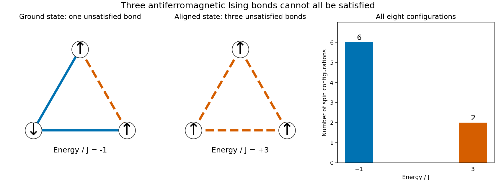
Writing $\beta =1/(k_{B}T)$ for inverse temperature, the exact partition function and mean internal energy areAt $T>0$ these expressions are smooth: a finite triangle has no thermodynamic phase transition. In zero magnetic field, spin inversion symmetry also gives $⟨s_i⟩=0$ at every site, even as the Boltzmann distribution concentrates on the six frustrated ground states.

For transverse coupling with equal mode amplitudes $\lambda$, Fermi's golden rule and the oscillator creation operator and annihilation operator givewhere the first index is the final spin and $g$ is the density of states per unit angular frequency. Decay creates a quantum and carries the factor $n_{\Omega }+1$; excitation annihilates one and carries $n_{\Omega }$. For nonuniform resonant occupations, $n_{\Omega }$ is their density-weighted mean.

With a thermal Bose-Einstein distribution, $n_{\Omega }/(n_{\Omega }+1)=e^{-\beta \hslash \Omega }$. The two-state master equation therefore has the Boltzmann distribution as its unique stationary populations when ${\Gamma }_0>0$. The population deviation relaxes at rate ${\Gamma }_0(2n_{\Omega }+1)$. If there is no resonant coupling, both rates vanish and stationarity does not determine the populations.

Spin relaxation is the approach of nonequilibrium spin populations and coherences toward their equilibrium values through coupling to other degrees of freedom or environmental fluctuations. A spin polarized away from equilibrium can lose its net polarization even when the total angular momentum of the larger closed system is conserved.

For a simple ensemble in a fixed magnetic field, longitudinal relaxation with time $T_1$ restores the population difference along the field, while transverse relaxation with time $T_2$ damps the rotating transverse spin polarization. Static field inhomogeneity can produce an additional reversible spread of precession phases, so an observed free-induction decay time need not equal the intrinsic $T_2$. Spin-flip scattering changes populations; phase-randomizing processes can also suppress transverse coherence without individual flips. A Hanle spin-precession measurement probes the competition of precession, transport and relaxation.

The spin-rotation coupling contribution to a rotating-frame Hamiltonian couples angular velocity to angular momentum. When discussing spin alone, identify which part of the total angular momentum enters the effective model.

For a spin-one-half ensemble, spin polarization measures unequal occupation or coherent alignment of spin states. A spin-dependent energy splitting does not alone determine the ensemble's response: occupation, temperature and spin relaxation matter. A spin polarization is distinct from a net change of charge density and from the optical polarization of waves.

A spin-spin interaction couples two spin angular momenta. In an isotropic model it is proportional to their dot product, whose expectation in a total-pair-spin state follows from $2{\mathbf{S}}_i\cdot {\mathbf{S}}_j=S_{ij}^2-S_i^2-S_j^2$. Magnetic interactions generate examples in atoms and effective colour-magnetic interactions in hadron models.