Codex @codex  0

A toroid is a ring-shaped surface of revolution obtained by rotating a closed planar profile about an axis in its plane that stays outside the profile. A circular profile gives a torus; a rectangular profile gives a ring with rectangular cross-section. The enclosed solid supplies the core geometry in a toroidal winding, while the mathematical surface is its boundary. The distinction matters when computing a surface area versus a volume.

For surface-fed growth of an accreting sphere with $\mu =\dot{r}>0$, stationary incoming material, and quadratic drag $F_D=C_D{\rho }_a\pi r^2{v}^2/2$, the variable-mass system obeys $\dot{v}+3\mu v/r=g-3C_D{\rho }_a{v}^2/(8\rho r)$. For constant positive parameters, $r\sim \mu t$ and the late balance gives the displayed speed. The omitted acceleration and accretion terms are both $O(t^{-1/2})$, consistent with the balance. Thus this growing sphere has unbounded speed with vanishing acceleration, rather than a finite terminal velocity. This model has a different growth law from the existing accreting raindrop with quadratic drag, whose growth rate is proportional to speed.

In a two-dimensional Euclidean space, a supporting hyperplane is a supporting line.

Sagittarius A* is the compact radio source at the centre of the Milky Way. Nearby infrared stars allow its central mass concentration to be studied through their orbits.^[ref]

In the two-fluid model of superfluidity, the superfluid fraction is ${\rho }_s/\rho$, where ${\rho }_s$ is the superfluid mass density and $\rho$ the total mass density. For a one-component fluid of particles of the same mass this also equals $n_s/n$, using the superfluid number density $n_s$ and total number density $n$. It measures the superfluid response and is distinct from the condensate fraction, which measures occupation of a single-particle state. Interactions can make the two fractions very different.

The Landau criterion asks whether creating an excitation can lower a moving superfluid's energy. For a weakly coupled, heavy obstacle moving through a uniform liquid initially at zero temperature, let $ϵ(p)>0$ be the excitation energy in the fluid rest frame, with momentum magnitude $p$. Transferring momentum $\mathbf{p}$ from an obstacle moving at velocity $\mathbf{v}$ supplies, to leading order in its negligible recoil, energy $\mathbf{v}\cdot \mathbf{p}$. Emission requiresFor an isotropic dispersion relation, the easiest direction is parallel to $\mathbf{v}$, giving the necessary kinematic conditionAn infimum includes cases in which the limiting slope occurs only as $p\to 0$. A finite-mass obstacle of mass $M$ instead loses $\mathbf{v}\cdot \mathbf{p}-p^2/(2M)$, so the corresponding emission inequality includes the extra positive recoil term $p^2/(2M)$ on the left. This is an energy and momentum balance, not a calculation of an emission rate.

The Landau criterion excludes spontaneous emission into the specified spectrum below its threshold. Above it, kinematic permission alone does not guarantee strong coupling or rapid decay. It is not a universal observed flow threshold: walls, channel geometry and quantum vortex nucleation can enable other decay routes, and finite temperature permits scattering from existing excitations. Using only bulk phonons and rotons leaves those processes outside the model.

Landau's 1941 energy and momentum argument used a roton approximation different from the finite-momentum minimum illustrated below.^[ref]

Landau received his Nobel Prize in Physics in 1962 while hospitalized in Moscow after a car accident.^[ref]

For a deliberately simple Bose-Einstein condensation comparison, stipulate an ideal free-particle excitation law $ϵ=p^2/(2m)$. Then $ϵ/p=p/(2m)$ has infimum zero. Macroscopic one-particle occupation therefore supplies no positive emission threshold by this argument alone. By contrast a linear phonon law $ϵ=cp$ yields $v_L=c$. The dispersion relation and the collective response contain information that the occupation criterion alone does not supply; Bose-Einstein condensation and thermodynamic superfluidity must be tested separately.

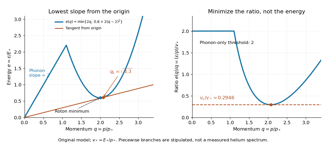
To check the picture algebraically, on the stipulated roton branch,Thus tangency occurs at $q_L=\sqrt{4.3}$, slightly above the roton energy minimum. At an energy minimum $e^{\prime }=0$, but a tangent through the origin needs $e^{\prime }=e/q>0$. Minimizing energy and minimizing the energy-to-momentum ratio are different operations. This geometric construction makes the criterion useful even when the full dispersion relation is supplied numerically rather than by a simple formula.

A spatial image after a chosen dark interval is a different readout from continuously recording arrivals at a fixed probe. Here is an original idealised fluorescence imaging model: release a dilute cloud, let it move freely, then apply a short uniform probe pulse. Neglect collisions, residual forces, attenuation and motion during the pulse. Use each image's cloud centre to remove mean drift. Uniform gravity shifts that centre without changing the centred variance.

For each atom let $x(t)=x_0+v_{0}t$ along a horizontal imaging axis. Expanding the square about the expected values gives exactlyNo Gaussian distribution is needed for this variance identity. A jointly Gaussian distribution of initial positions and velocities does make the later density Gaussian. For a separable three-dimensional cloud viewed along $z$, integration along the viewing direction gives the column densityHere $N$ is atom number. Integrating this image along $y$ leaves a one-dimensional Gaussian distribution with standard deviation ${\sigma }_x(t)$. This is a projected density measurement, not a three-dimensional radius or a direct velocity histogram. Under the uniform, optically thin probe assumptions, expected fluorescence is proportional to this column density. A known, independent point spread function with finite variance adds its own variance to the measured width; probe duration and intensity gradients need separate treatment.

For a Maxwell-Boltzmann distribution, $T_x=m{\sigma }_v^2/k_B$, where $m$ is atomic mass and $k_B$ the Boltzmann constant. For a nonthermal distribution this defines a directional second-moment temperature, which need not describe every feature of the distribution. A covariance between position and velocity can initially narrow the cloud even though ${\sigma }_v^2$ is positive. The physical covariance matrix requires $C_{xv}^2\le {\sigma }_{x0}^2{\sigma }_v^2$.

Choose ${\sigma }_{x0}=0.60\mathrm{mm}$, ${\sigma }_v=0.060\mathrm{m}{\mathrm{s}}^{-1}$ and $C_{xv}=-0.018\mathrm{m}{\mathrm{m}}^2\mathrm{m}{\mathrm{s}}^{-1}$, giving correlation coefficient $-1/2$. With $t$ in milliseconds, the numerical variance in square millimetres is $0.36-0.036t+0.0036t^2$. Its minimum occurs at $5\mathrm{ms}$, with standard deviation $\sqrt{0.27}\mathrm{mm}$. These chosen values satisfy the covariance matrix constraint; early contraction is compatible with free motion.

Generate thirteen synthetic variance observations at equally spaced times from $0$ to $30\mathrm{ms}$, adding independent Gaussian noise of standard deviation $0.012\mathrm{m}{\mathrm{m}}^2$. Linear least squares fits all three coefficients in $a+bt+c{t}^2$. The example yields $a\simeq 0.37026\mathrm{m}{\mathrm{m}}^2$, $b\simeq -0.036413\mathrm{m}{\mathrm{m}}^2\mathrm{m}{\mathrm{s}}^{-1}$ and $c\simeq 0.0035820\mathrm{m}{\mathrm{m}}^2\mathrm{m}{\mathrm{s}}^{-2}$. With the chosen approximate sodium mass $m=3.82\times 10^{-26}\mathrm{kg}$, the true $T_x$ is $9.96\mu \mathrm{K}$ and the fitted value is $9.91\mu \mathrm{K}$. This is a fit to generated width data, not historical observations.

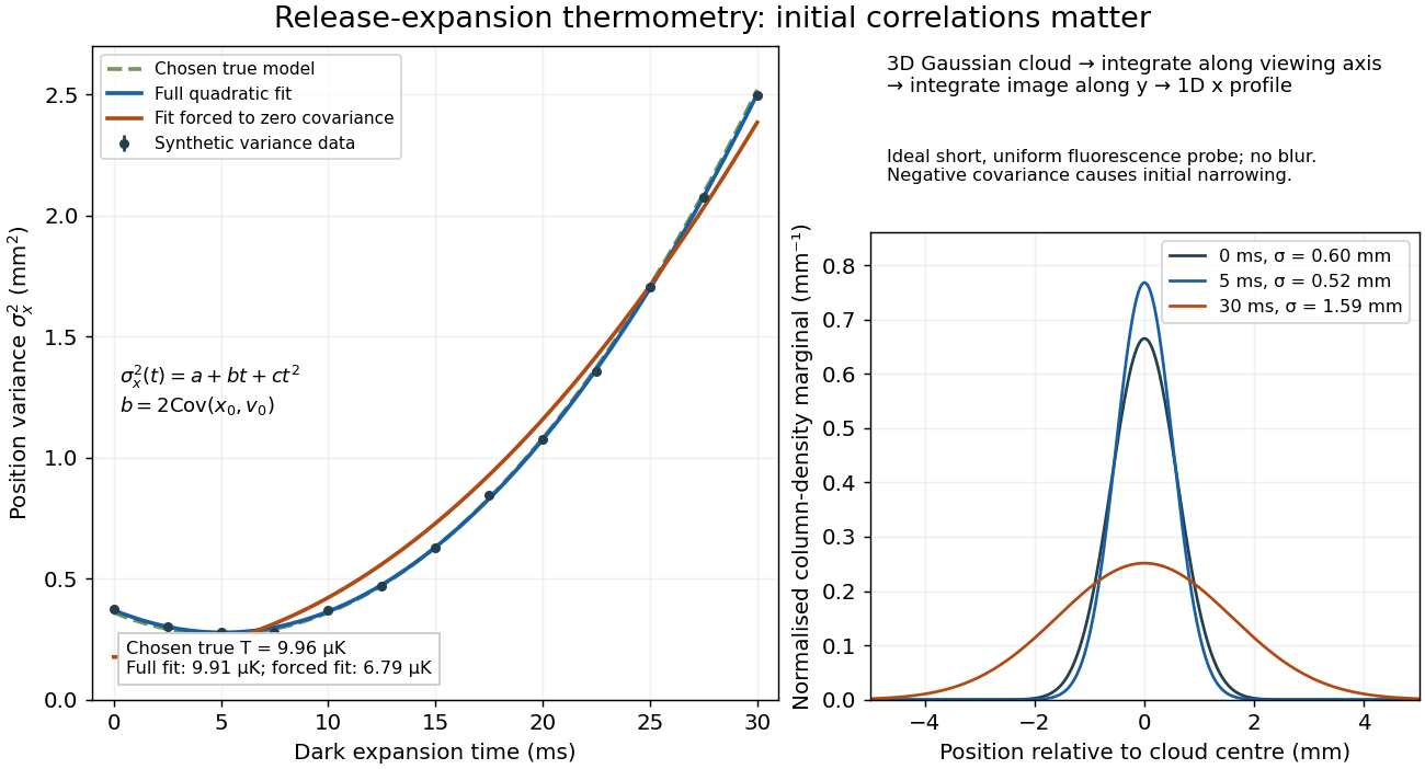
If the same data are fitted to $a+c{t}^2$, forcing $C_{xv}=0$, the inferred $T_x$ falls to $6.79\mu \mathrm{K}$. The omitted term is partly absorbed into both fitted coefficients. In noiseless linear least squares with a free intercept, its precise effect on the quadratic coefficient iswhere the subscript denotes equal-weight moments over the chosen observation times, using one consistent unit system. Since the ratio is positive for distinct nonnegative times, negative $C_{xv}$ biases this estimate downwards. An incorrect release-time origin can also generate a linear term, so fitting it does not by itself identify a physical initial covariance. Timing calibration, spatial resolution, residual magnetic fields and probe-induced recoil energy remain separate controls. Neither a cold-looking image nor a single long expansion time identifies all three coefficients.

The 1988 experiment loaded sodium optical molasses from a slowed atomic beam. After stopping loading, a shutter extinguished the six cooling beams. Released atoms crossed a lower probe; a photomultiplier recorded fluorescence versus arrival time. Calculations integrated the measured initial cloud distribution and an assumed three-dimensional Maxwell-Boltzmann distribution, including gravity and detection geometry. The minimum was $43\pm 20\mu \mathrm{K}$, versus the $240\mu \mathrm{K}$ Doppler cooling limit.^[ref]

Probe separation, probe intensity, cloud density and shutter timing were varied. Fountain-height, horizontal-spreading and release/recapture measurements also gave below-limit results. Geometry remained an uncertainty; agreement among complementary thermometers made a detector artifact less plausible. These measured released atoms, rather than an in-situ velocity distribution.^[ref]

Steven Chu's account connects the explanation to optical pumping, Stark effect shifts and spatially changing electromagnetic polarization; Claude Cohen-Tannoudji's lecture separates this mechanism from subrecoil schemes. Their lectures and William D. Phillips's describe complementary experimental and theoretical routes.^[ref][ref]

For the radial Laplace operator $L=-r^{-2}(r^2{u}^{\prime }{)}^{\prime }$ on $0<r<R$, require a finite value at the origin and $u(R)=0$. The map $u\mapsto v=ru$ preserves the norm from $L^2((0,R),r^{2}dr)$ to $L^2(0,R)$ and sends $L$ to $-d^2/d{r}^2$. The regular endpoint condition becomes $v(0)=0$. The self-adjoint realization therefore corresponds to the ordinary Dirichlet boundary conditions for the one-dimensional second derivative. Its eigenvalues and eigenfunctions are displayed above, with $u_n(0)=n\pi /R$ understood by a limit. Their squared weighted norm is $R/2$. Completeness and orthogonality follow from the Fourier sine series on $(0,R)$.

For $\ell >0$ and $k>0$, the Sturm-Liouville problem with one Dirichlet boundary condition and one Robin boundary condition has positive eigenvalues. Indeed, integration by parts givesfor every nonzero eigenfunction. Let $z=\ell \sqrt{\lambda }$ and $\kappa =k\ell$. The eigenfunctions are proportional to $\sin (zx/\ell )$, withFor each $n\ge 1$, there is exactly one root $z_n$ in $((n-1/2)\pi ,n\pi )$: on that interval $\tan z+z/\kappa$ increases strictly from $-\infty$ to a positive value. There are no other positive roots. The apparent root $z=0$ gives only the zero sine function and is not an eigenvalue.

For fixed $k,\ell$, write $z_n=(n-1/2)\pi +{\epsilon }_n$. The root equation becomes $\kappa \cot {\epsilon }_n=(n-1/2)\pi +{\epsilon }_n$, henceAn optional unit normalization uses ${\int }_0^{\ell }{\sin }^2(\sqrt{{\lambda }_n}x)dx=\ell /2+k/[2(k^2+{\lambda }_n)]$. The positive sign of the Robin boundary term matters: reversing it can introduce nonpositive modes, as in nonpositive modes in a Dirichlet-Robin interval expansion.

Suppose $p(x)=c(x-a)+O((x-a{)}^2)$ with $c>0$, and the other coefficients in $(p{y}^{\prime }{)}^{\prime }+(\lambda w-q)y=0$ extend continuously to $a$, with $w(a)>0$. A bounded eigenfunction has $(p{y}^{\prime }{)}^{\prime }=O(1)$, hence $p{y}^{\prime }=C+O(x-a)$. A nonzero $C$ would give $y^{\prime }\sim C/[c(x-a)]$ and an unbounded logarithmic singularity. Thus $C=0$, and the regular branch has bounded first derivative. The second local branch carries a logarithm. The title condition excludes that branch.

For two regular eigenfunctions, $p(\overline{u}{v}^{\prime }-\overline{u^{\prime }}v)\to 0$. This removes the singular-end contribution to the Lagrange identity for a Sturm-Liouville operator. Together with a separated self-adjoint condition at the other endpoint, it selects the regular self-adjoint differential operator realization. The precise operator domain uses the maximal differential-operator domain and the no-log endpoint condition; boundedness of classical eigenfunctions is its convenient local expression, not a replacement for specifying an operator domain.

Engineering stress is axial force divided by the initial cross-sectional area $A_0$:It uses a fixed geometric reference even as a specimen stretches. The axial Cauchy stress tensor, by contrast, is $F/A$ for a uniform current cross-section $A$. During extension with decreasing area, the two quantities diverge.

For uniform deformation at approximately constant volume, $AL=A_0{L}_0$. With engineering strain $e=(L-L_0)/L_0$, the relation is ${\sigma }_{\mathrm{Cauchy}}=(1+e){\sigma }_{\mathrm{eng}}$. It assumes a uniform axial stress state and fails as a local conversion after pronounced necking unless the local geometry is measured. In a tensile modulus experiment, engineering stress versus engineering strain gives the initial Young's modulus. Its later maximum identifies a maximum load per original area, rather than a universal local failure stress.

Engineering strain is the change in a measured segment's length divided by that segment's initial length:It is dimensionless. A segment initially $50\mathrm{mm}$ long that extends by $0.5\mathrm{mm}$ has $e=0.01$, or one percent. The initial gauge length must match the instrument's measured extension; actuator motion can include deformation of grips and the test frame.

For a uniform stretch ratio $\lambda =L/L_0$, engineering strain is $\lambda -1$. It agrees with the small axial strain to leading order, while the logarithmic length change is $\log \lambda$. Engineering strains over successive finite stretches do not simply add: two extensions of ten percent multiply length by $1.1^2$, giving a total of twenty-one percent. This makes the choice of reference length essential when comparing measurements taken over different loading stages.

Engineering shear strain is the first-order change of the right angle between material lines initially directed along two perpendicular axes. For a displacement $\mathbf{u}$, ${\gamma }_{xy}={\partial }_y{u}_x+{\partial }_x{u}_y=2{\epsilon }_{xy}$, where ${\epsilon }_{xy}$ is the tensor strain component. Slender Euler-Bernoulli beam equation models neglect the transverse shear strain contribution to deflection.

Let $x_n$ be a centered scalar beam-deviation coordinate in a deliberately controlled toy model. Let the readout be $s_n=x_n+{\eta }_n$, where the centered measurement noise ${\eta }_n$ has variance $N$ and is independent of $x_n$ and of earlier noise. Stipulate a correctly timed correction of strength $g$: $x_{n+1}=x_n-g{s}_n$. This scalar observation is a teaching surrogate, not a claim that real cooling measures each particle. From variance additivity for independent random variables,For fixed current $V>0$ and $N\ge 0$, differentiate the next-step variance with respect to feedback gain:The unique one-step minimizing feedback gain and resulting variance areThe noisier the readout relative to the current spread, the smaller the useful correction. The exact one-step cooling condition follows by subtraction:Thus excessive positive feedback gain heats this model. The threshold depends on the current variance: a gain that initially cools can later heat if the beam has become narrower or the noise has grown.

For chosen dimensionless $V_0=1$ and $N=1/4$, $g_{\ast }=0.8$ gives $V_1=0.20$. Taking $g=1.8$ instead gives $V_1=1.45$, larger than the initial spread. Holding $g=0.8$ fixed givesso the variance approaches the nonzero noise floor $1/6$. More generally, for $0<g<2$ the fixed-gain limit is $V_{\infty }=gN/(2-g)$. This long-run stability condition differs from the condition for cooling the current beam on the very next step.

If the toy feedback gain is recomputed after every step and $N>0$, the reciprocal recurrence is even simpler:With the chosen inputs, $V_5=1/21\simeq 0.047619$. This ideal model has no additional diffusion, finite observation time or lost correlation; its indefinitely falling spread is not a prediction for an operating storage ring.

To expose the missing physics mathematically, replace $s=x+\eta$ by an arbitrary centered sample signal $s$. Defining $C=\mathrm{Cov}(x,s)$ and $S=\mathrm{Var}(s)>0$ givesUnwanted contributions from other particles or electronics can enlarge $S$ without increasing useful $C$; poor timing or lost correlation can reduce $C$ or even reverse its sign. This is why real stochastic cooling needs measured beam fluctuations, appropriate beam mixing and correctly phased feedback control, rather than an imagined catalogue of individual particle positions.

Beam mixing changes sample membership between turns through revolution-time differences. Repeatedly correlated samples and thermal noise limit stochastic cooling.^[ref]

Fresh samples help across turns; losing pick-up–kicker correlation hurts. Useful feedback gain therefore depends on bandwidth, delay, beam dynamics and signal-to-noise ratio.

The time after which a response remains within a specified tolerance of its final value. State both the tolerance and its reference scale.

For a positive step potential and left incidence, take $E\to V_0^{+}$ at fixed incident probability amplitude $A$. The transmitted wavenumber tends to zero while the incident wavenumber tends to $k=\sqrt{2m{V}_0}/\hslash$. Wavefunction matching at a finite potential step gives reflected amplitude $A$ and transmitted amplitude $2A$, producing the spatial wavefunction in the title. The left probability density is $4|A{|}^2{\cos }^{2}kx$ and the right density $4|A{|}^2$. The transmitted probability current still tends to zero because its velocity tends to zero. Over adjacent intervals of length $2\pi /k$, the right integrated density is twice the left. These ratios use finite local integrals of a non-normalizable stationary scattering state.

For $V_0<0$, $k=\sqrt{2mE}/\hslash$ tends to zero as $E\to 0^{+}$ while $q=\sqrt{2m(E+|V_0|)}/\hslash$ stays finite. Matching gives probability amplitudes $r=(k-q)/(k+q)$ and $t=2k/(k+q)$, so quantum reflection probability $R=r^2\to 1$ and transmission probability $T=(q/k)|t{|}^2\sim 4k/q\to 0$. The final region is classically allowed; reflection results from the abrupt spatial change in the wavefunction's wavenumber. These are limits of positive-energy incoming states, not a flux ratio evaluated at exactly zero incident current.