
Work by Ryohei Yasuda Created 2026-10-18 Updated 2026-11-05
ER signal sequence 2026-10-18
An ER signal sequence is polypeptide chain targeting information recognized by machinery delivering a protein to the endoplasmic reticulum. Many soluble cargoes have a removable N-terminus signal; membrane insertion can use internal signals. An ER signal sequence alone does not specify the final destination.[ref]
The Endoplasmic Reticulum. Molecular Biology of the Cell, 4th edition by Bruce Alberts and others; The ER Signal Sequence Is Removed from Most Soluble Proteins After Translocation; In Single-Pass Transmembrane Proteins, a Single Internal ER Signal Sequence Remains in the Lipid Bilayer as a Membrane-spanning α Helix
For an original counting example, stipulate an unbranched precursor polypeptide chain of amino acid residues whose first amino acid residues form a cleaved ER signal sequence. With no further processing, the remaining chain has amino acid residues and peptide bonds. The initial chain had peptide bonds; the detached signal has , so remain after one bond is cut. The check counts adjacent positions: an unbranched chain of amino acid residues has peptide bonds. These stipulated lengths are not a natural sequence, a measured size or evidence that a particular sequence functions as an ER signal sequence.
Real rotation matrices that are Hermitian Created 2026-10-18 Updated 2026-10-20
A real rotation matrix is a unitary matrix because it is an orthogonal matrix. It is a Hermitian matrix precisely when it is symmetric, equivalently when its square is the identity. Its eigenvalues are then . In three dimensions a proper rotation is therefore Hermitian only for the identity or a half-turn. A half-turn about a unit vector has matrix : it fixes and reverses the perpendicular plane. For every real rotation , the difference is anti-Hermitian; it is also Hermitian only in the zero case.
Work by Ronald Alfred Laskey 2026-10-18
Spring-mounted rolling cylinder Created 2026-10-18 Updated 2026-10-20
Attach a spring of spring constant to the axle of a round body of mass , radius and axial moment of inertia . Assume rolling without slipping, a horizontal drag force applied through the axle, and no additional resisting torque. The translational force equation is , where is signed static friction. The rotational equation and rolling constraint give , yielding the displayed equation. Equivalently, the kinetic energy is . This added effective inertia lowers the undamped angular frequency to . A distributed viscous torque would add a separate damping term and cannot be inferred from the drag force alone.
Work by Rodney Robert Porter 2026-10-18
Work by Robin Hill 2026-10-18
Quantum covariance 2026-10-18
For self-adjoint operators and an admissible pure state, the quantum covariance is the real, symmetrized second moment of two centered observables. The displayed expression uses their anticommutator; equivalently , which requires only the individual finite second moments. It reduces to ordinary covariance for commuting observables. For noncommuting observables, its definition does not assert that both have simultaneous sharp values drawn from a joint classical probability distribution.
Work by Robert K. Nakamoto Created 2026-10-18 Updated 2026-10-31
Work by Robert F. Cook 2026-10-18
Work by Robert Brown Created 2026-10-18 Updated 2026-11-05
Rindler null geodesics Created 2026-10-18 Updated 2026-10-25
For in a patch with , the null paths solve , giving with . They are geodesics after choosing an affine parameter. The Rindler coordinates , give and . Thus each exponential path is a straight inertial null line. A literal curve is outside this degenerate coordinate chart, not an extra null geodesic within it.
Work by Rikiya Watanabe Created 2026-10-18 Updated 2026-10-31
Line element Created 2026-10-18 Updated 2026-10-20
The line element of a Riemannian metric is its local expression for squared infinitesimal length. Along a parametrized curve , the arc length is . For a circular cylinder of radius parametrized by angle and axial position , the induced metric gives . Unrolling with yields the Euclidean form , explaining the straight unrolled descriptions of geodesics on a circular cylinder.
Thermionic tail-flux derivation Created 2026-10-18 Updated 2026-10-20
Consider a planar surface with outward normal along . For an auxiliary equilibrium electron gas just outside it, let be the total number density, counting both signs of . Its Maxwell-Boltzmann velocity distribution has normal-component densityAn electron with crosses more area per unit time when it moves faster. The outgoing number flux therefore uses , rather than just the probability of :This integral contributes only . Holding a classical bulk number density fixed and imposing a normal kinetic energy threshold would instead give ; that argument alone does not produce .
For the ideal surface model, measure external electron energies from the metal's chemical potential . A freely propagating external state has . When , its Fermi-Dirac distribution reduces to the Maxwell–Boltzmann statistics tail. Counting two spin states per phase space cell of volume givesEach of the three Gaussian integrals supplies . Combining this state count with the crossing factor givesThe auxiliary atmosphere supplies an equilibrium state-counting argument; an operating collector removes the outgoing electrons. It need not maintain a real equilibrium gas throughout the gap. Unit transmission and the ideal free electron state count are substantive assumptions, so this calculation does not determine an arbitrary real surface's measured .
In particular, electrons inside a metal generally form a degenerate Fermi gas. A classical distribution for the escaping tail does not imply a classical distribution for the whole interior. Richardson himself emphasized this distinction in his lecture.[ref]
Thermionic Phenomena and the Laws which Govern Them by Owen Willans Richardson. Nobel Lectures, Physics 1922–1941; pp. 230–231, internal versus external electron statistics
Richardson plot 2026-10-18
Choose a fixed positive reference with the same units as . Taking the natural logarithm of a dimensionless ratio givesThus the Richardson plot is a straight line when and are constant, with slope and intercept . The familiar notation silently chooses units; the reference makes that choice explicit. Changing shifts the intercept and leaves the inferred work function unchanged. If the horizontal axis instead uses , its slope is .
For the chosen example, choose . Then and . Their slope is approximately , giving . Two temperatures determine a line algebraically; several temperatures allow curvature and drift to be detected. These values are calculated, rather than experimental observations.
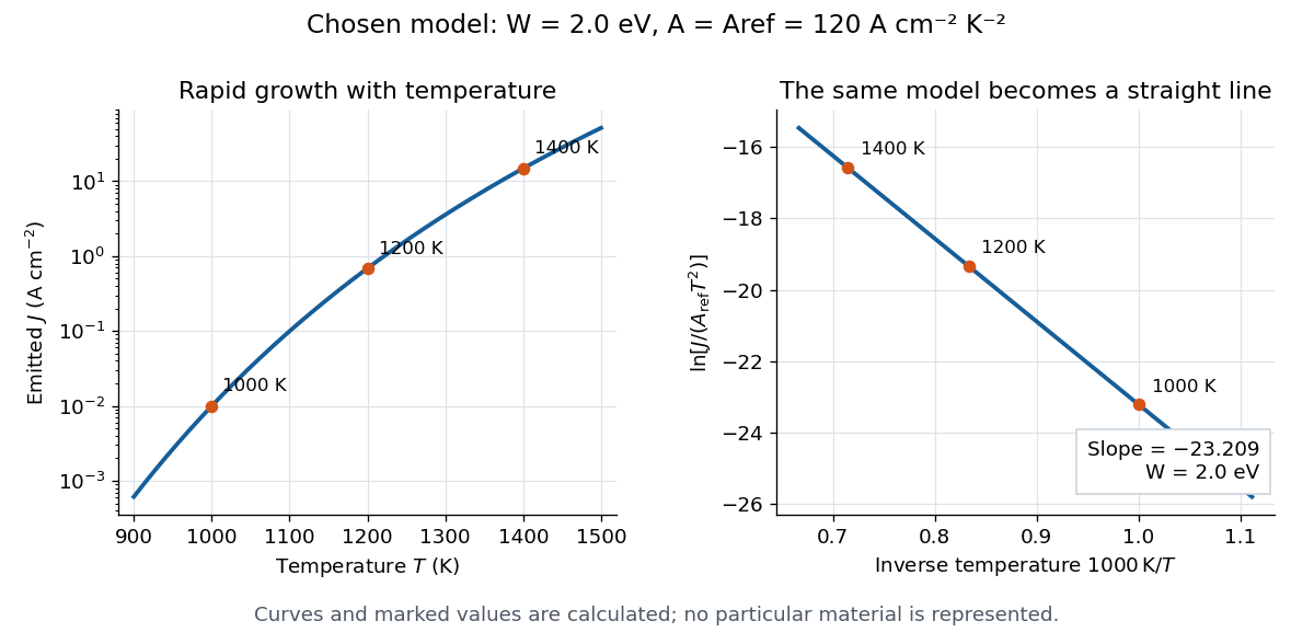

A straight trace alone does not establish a unique surface work function. Adsorption, changing surface coverage, or a mixture of regions with different barriers can change the inferred slope. For independent emitting patches with area fractions , constant and barriers ,Lower barriers contribute disproportionately. Even with fixed patches, the slope of the Richardson plot gives a temperature-dependent weighted mean of the , rather than their simple area average. If or themselves vary with temperature, the apparent slope-derived barrier becomesCheck collection, temperature calibration, and surface stability before assigning curvature to a new emission mechanism.
Thermionic Richardson constant Created 2026-10-18 Updated 2026-10-20
The coefficient has dimensions of electric current density divided by squared temperature. For ideal nonrelativistic particles with the free electron mass, two spin states, a planar uniform surface, and unit escape transmission, the thermionic tail-flux derivation giveswhere is the positive elementary charge and is the Planck constant. The two area units differ by a factor of . A fitted need not equal : reflection at the surface, the electronic band structure, and uncertain emitting area affect the inferred coefficient. A constant escape transmission would give in this simple model; an energy-dependent transmission generally requires an integral instead.
The name joins Owen Willans Richardson with Saul Dushman. Dushman's 1923 paper develops a thermodynamic treatment of electron emission analogous to evaporation and evaluates the prefactor using quantum ideas.[ref]
Electron Emission from Metals as a Function of Temperature by Saul Dushman. Abstract, general equation and theoretical evaluation of A
Eliminating a variable with a resultant 2026-10-18
Consider the original pair of polynomial equationsTreat them as polynomials in with coefficients in . Their Sylvester matrix and resultant areEvery common solution must therefore have or . Back-substitution into gives , and both pairs also satisfy . The complete real solution set isHere elimination and direct substitution agree: subtracting from gives , exactly the same condition.
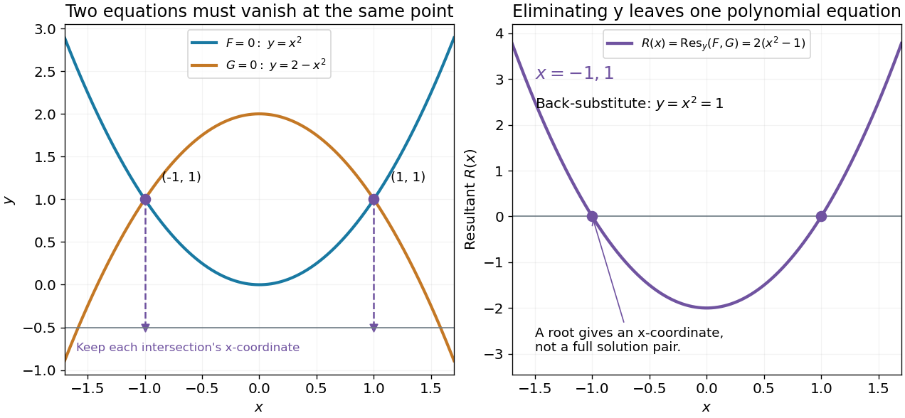
Polynomial elimination keeps the possible first coordinates of intersections
. Original parabola example. Left: both equations vanish at the two marked intersections; dashed lines retain their -coordinates on an auxiliary horizontal reference line at . Right: the resultant has zeros at those coordinates. Substitution recovers and verifies each full solution pair. Details.
In general, first solve the one-variable resultant equation, then recover and check the other coordinate in both original polynomial equations. A real coordinate candidate can correspond only to nonreal values of the eliminated variable. Also, vanishing leading coefficients require the separate check in degree drop in a specialized resultant. The general elimination-and-back-substitution method is described in the lecture's §3.1.[ref]
Lecture 6: Resultants and Discriminants. Algebraic Techniques and Semidefinite Optimization, MIT 6.972, Spring 2006; MIT 6.972, Lecture 6, p. 6-3, §3.1 Polynomial equations: eliminate one variable, solve and back-substitute
Resultant as a product over roots 2026-10-18
Write and in an algebraic closure, counting multiplicity of a root. The coefficient-row convention above givesThis makes the shared-root of a polynomial test transparent: a factor vanishes precisely when one equals one . Swapping the two polynomials reverses the sign of all differences, giving .[ref]
The value measures an algebraic product, not a normalized geometric distance. Replacing by for nonzero leaves its roots of a polynomial unchanged but multiplies the resultant by . Therefore a small numerical resultant alone does not quantify how close two sets of roots of a polynomial are. Exact zero testing and numerical sensitivity are different questions.
A multiple root of a polynomial is also a root of a polynomial of its formal derivative. In characteristic zero, for , the associated discriminant isFor example, gives and . The two roots of a polynomial merge precisely at .[ref]
Lecture 6: Resultants and Discriminants. Algebraic Techniques and Semidefinite Optimization, MIT 6.972, Spring 2006; MIT 6.972, Lecture 6, p. 6-2, Definition 2: discriminant as a polynomial–derivative resultant
Respiratory control ratio 2026-10-18
The respiratory control ratio divides the oxygen consumption rate during ADP-stimulated respiration by that after supplied ADP has been used. It compares reaction rates, not ATP formed per oxygen.[ref]
Respiratory enzymes in oxidative phosphorylation. I. Kinetics of oxygen utilization by Britton Chance and G. R. Williams. pp. 386–387, Figure 2 and discussion of the ratio of respiration rates with and without ADP
A large ratio means strong stimulation under the comparison's conditions; it is not a universal measure of all mitochondrial functions.
For a constructed example, choose constant suspension volume and oxygen concentration declines of and during the two comparison windows. Assume no gas exchange or dilution and a correctly calibrated readout. A derivative converts each concentration slope into an amount of substance consumption rate:The common volume cancels in the ratio, so dividing the positive slope magnitudes gives the same answer. These are chosen inputs, not the 1955 observations. If an uncorrected influx of of oxygen occurred in both windows, the apparent rates would instead be and , giving . The same absolute error can inflate a ratio because it removes a larger fraction of its smaller denominator.
There are unlisted articles, also show them or only show them.