
Nuclear mass parabola 2026-10-18
At fixed mass number , the smooth semi-empirical mass formula makes the atomic mass approximately quadratic and convex in atomic number . Neighboring nuclear isobars undergo energetically allowed beta decay toward a discrete local minimum, subject to the electron-mass threshold for beta-plus decay. For odd there is one smooth branch; for even , nuclear pairing splits the even-even and odd-odd branches. A local minimum against a single change of need not be stable against double beta decay.
Nuclear Coulomb energy 2026-10-18
Nuclear Coulomb energy is the positive electrostatic mass-energy contribution from proton repulsion in a nucleus. A uniform-charge model gives scaling , and approximately constant nuclear density gives . It reduces conventional positive nuclear binding energy.
Beta decay Q values depend on small differences between much larger atomic masses. A smooth semi-empirical mass formula can therefore approximate absolute masses reasonably while predicting the wrong sign for a MeV-scale decay threshold. Nuclear pairing explains offset even-even and odd-odd mass branches, but does not guarantee that every specific even-even neighbor lies below the intervening odd-odd nucleus. Measured masses or additional nuclear shell corrections are needed for quantitative threshold tests near a model's residual error scale.
For a spherical self-similar blast wave, put , , and . The radial Euler equation then requires , whereThis follows from and . The momentum equation alone leaves a spatially uniform additive pressure undetermined. The scale-free strong-shock boundary data fix that freedom consistently with the displayed similarity scaling; an independently prescribed ambient pressure introduces another scale.
Use the fields of pressure similarity in a spherical blast wave, with front radius . Since , changing the radial integration variable to givesBoth are time independent for fixed integrable similarity profiles and constant front coordinate . With explosion energy and negligible external energy input or losses, their sum equals . This normalization, together with shock matching and regularity, fixes the dimensionless blast coefficient rather than dimensional analysis alone.
Sedimentation equilibrium Created 2026-10-18 Updated 2026-11-05
Sedimentation equilibrium occurs when the downward tendency of suspended particles is balanced by their diffusion, leaving a stationary concentration profile with no net particle flux. For dilute identical particles in an isothermal fluid, let be their buoyant mass. Balancing the gradient of ideal osmotic pressure against gravity givesHere height increases upward, and heavy particles have .
The profile is a miniature atmosphere: thermal motion spreads particles upward while gravity favours lower positions. The Perrin sedimentation experiment measured particle counts at different microscope focal heights and used this competition to infer a molecular energy scale.[ref]
Mouvement brownien et réalité moléculaire by Jean Baptiste Perrin. 1909 memoir, §§15 and 20–22, vertical grain populations and tests using independently measured grain properties
A stationary profile requires sufficiently slow background flow and controlled temperature; a growing deposit during ongoing settling is a different situation.In 1967, James D. Jamieson and George E. Palade incubated guinea pig pancreas slices, following a three-minute pulse of tritium-labeled leucine with excess unlabeled leucine. This pulse-chase analysis marked newly made proteins while reducing subsequent incorporation. Fixed, Epon-embedded thin sections were mounted on coated grids, covered with Ilford L-4 photographic emulsion, developed and stained for electron microscopy. Autoradiography located photographic grains relative to pancreatic acinar cell structures.[ref]
Intracellular Transport of Secretory Proteins in the Pancreatic Exocrine Cell. II. Transport to Condensing Vacuoles and Zymogen Granules by James D. Jamieson and George E. Palade. Jamieson and Palade, Intracellular Transport of Secretory Proteins in the Pancreatic Exocrine Cell. II. Transport to Condensing Vacuoles and Zymogen Granules (1967), p. 598 Methods; Figure 10: three-minute pulse
Pulse-end samples provided a temporal reference: label lay mainly over rough endoplasmic reticulum; later samples shifted toward peripheral Golgi apparatus elements, condensing vacuoles and secretory granules. As a contamination check, isolated granule pellets were also examined by autoradiography: early pellet labeling chiefly marked condensing vacuoles. Grids from the compared pellet samples were coated together to control photographic processing. This supported transport of a previously labeled cohort rather than separate synthesis at each location. Fixed samples did not track individual proteins; localization was finite, and labeling was not absolutely exclusive to secretory cargo. The result concerns this preparation, not every protein in every biological cell.[ref]
Intracellular Transport of Secretory Proteins in the Pancreatic Exocrine Cell. II. Transport to Condensing Vacuoles and Zymogen Granules by James D. Jamieson and George E. Palade. pp. 603–606 and Figures 10–13: changing localization; pp. 610–611 and Figures 14–15, Table III: pellet check and matched emulsion processing; p. 611 General Premises: nonexportable-protein labeling
For a classical dilute gas with pair potential for and zero otherwise, put . Substitution in the Mayer f-function formula givesIt is positive for finite positive temperature, tends to as in the classical model, and behaves as at high temperature. The low-temperature mathematical limit need not remain in the dilute classical regime for a real molecular gas.
Exchange contribution to the second virial coefficient Created 2026-10-18 Updated 2026-10-20
For a single internal species of noninteracting particles with quadratic dispersion in three dimensions, expand the grand canonical partition function at small quantum gas fugacity. With for bosons and for fermions, and . Eliminating gives . Bosonic bunching lowers the pressure at fixed density; fermionic exclusion raises it. This correction needs no interaction potential. For equally populated internal species, the coefficient in terms of total number density is reduced by . In the dilute one-species limit the equal-time pair detection correlation is . The exchange contribution to the two-particle cluster integral is therefore , providing a direct pair-counting check of the coefficient.
Phase matching in second-harmonic generation 2026-10-18
Phase matching makes wave amplitudes emitted at different depths add coherently. Consider collinear plane waves in a uniform transparent material of length , with fixed polarization of waves and nonzero selected nonlinear optical susceptibility. Assume negligible pump depletion, negligible absorption, an initially absent harmonic, and a wide beam for which diffraction is negligible. The pump's wave amplitude is then constant throughout the interaction.
The pump electric field has spatial wave phase ; its quadratic source has spatial wave phase . The freely propagating harmonic has wave number . Define the second-harmonic phase mismatch byFor the chosen complex-field convention, the outgoing harmonic wave amplitude, up to an overall constant and propagation phase, is proportional toChoosing the conjugate complex-field convention reverses the exponent's sign without changing the wave intensity. Taking the squared complex modulus givesHere is fixed for the chosen modes and material; its dimensions accommodate the stated wave intensity convention. The quadratic pump dependence follows because the source wave amplitude is proportional to , whereas is proportional to . The sinc function comes from summing contributions along the whole material, just as a finite aperture produces diffraction through addition of complex amplitudes.
At , the integral is and the harmonic wave intensity grows as . At , all those contributions cancel. This cancellation needs no absorption: their wave phases wind through a full turn. At high conversion, the constant-pump assumption fails, so the law cannot continue indefinitely. Tight focusing, finite optical pulses, absorption, and transverse separation of modes also require a more complete model.
Optical dispersion generally makes . In a suitable crystal, birefringence allows modes with different polarization of waves to experience different refractive indices, making their selected values equal. The appropriate crystal direction and allowed nonlinear optical susceptibility component must both work.[ref]
Nonlinear Optics and Spectroscopy by Nicolaas Bloembergen. p. 19: momentum mismatch and birefringence compensation
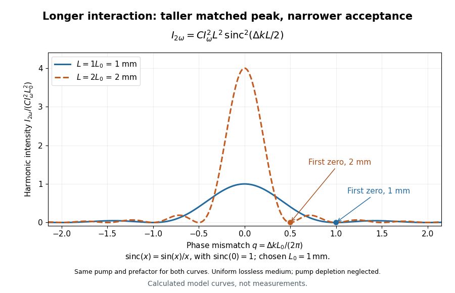

For a worked calculation, choose and . At , the harmonic wave intensity is of its perfectly matched value. At it vanishes in this model. More material can therefore reduce the output. If instead , doubling multiplies output by four. The two curves retain that common normalization, so their different peak heights are meaningful.
Franken and colleagues frequency-doubling experiment Created 2026-10-18 Updated 2026-10-20
In 1961, Peter Alden Franken, Alan Hill, C. Wilbur Peters and Gabriel Weinreich focused a pulsed ruby laser through a red optical filter into quartz. The filter suppressed xenon-flash background. A quartz-prism spectrograph used red-insensitive Eastman Type 103 plates. A single shot recorded a feature near from input. Removing the quartz or substituting glass removed the feature; changing polarization of waves and orientation followed their predicted pattern. These controls supported second-harmonic generation; photographic density gave an estimated yield.[ref]
Generation of Optical Harmonics by Peter Alden Franken and others. pp. 118–119, Table I, Fig. 1 and controls
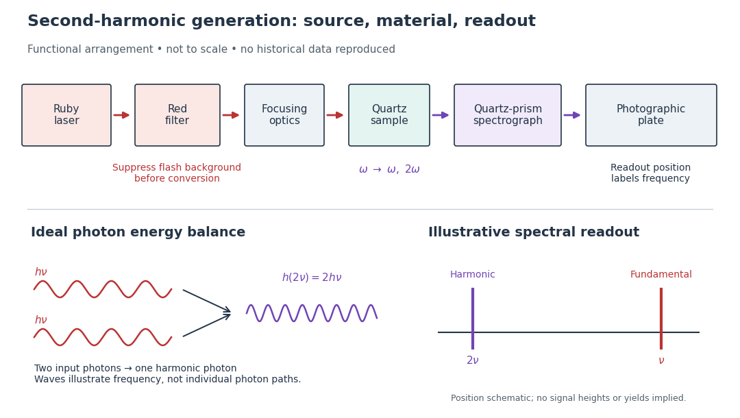

A spectrograph turns output frequency into a recording position. Its spectral separation makes a faint new component distinguishable from bright input light. The reported rounded wavelengths do not constitute an independent precision measurement of the ratio two. Nor do these observations demonstrate perfect phase matching or complete conversion. The experiment and Nicolaas Bloembergen's later theoretical account are distinct contributions to nonlinear optics.
Eddington experiment Created 2026-10-18 Updated 2026-10-25
The 1919 solar eclipse expeditions organized by Frank Watson Dyson and Arthur Eddington compared background-star positions near the obscured Sun with reference photographs. The optical train used a slowly rotating flat mirror to send the light into a horizontal photographic telescope. A smaller telescope at Sobral provided a separate set of plates. Focus and plate-scale changes had to be distinguished from the radial pattern predicted by Schwarzschild light deflection. The experiment therefore tested a spatial pattern and its amplitude, not merely whether a star image had moved.[ref]
A determination of the deflection of light by the Sun's gravitational field by Frank Watson Dyson and others. 1920 report of the 1919 observations
[ref]https://www.royalobservatorygreenwich.org/articles.php?article=1283. Equipment taken and the Sobral expedition: horizontal telescopes, tracking mirrors and reference plates
Babinet's principle 2026-10-18
In linear scalar diffraction theory, complementary aperture transmissions and give complex fields , where is the unobstructed field under identical illumination. Away from the direct beam in Fraunhofer diffraction, their diffracted fields differ by a sign and have equal intensity. Intensities do not generally add: in particular, complementary on-axis Fresnel diffraction patterns need not have equal intensity. The ideal scalar statement does not incorporate vector boundary details at a real conducting edge.
Work by Saurabh Upadhyay 2026-10-18
Sanger-Nicklen-Coulson sequencing experiment 2026-10-18
In 1977, Frederick Sanger, S. Nicklen and Alan Coulson tested chain termination on Phi X 174 DNA. They isolated restriction enzyme fragments as primers, heated them with template to for three minutes and annealed at for thirty minutes. Four extension mixtures used the Klenow fragment of DNA polymerase and radioactive dATP. Their Figure 1 used ddGTP, ddATP, ddTTP and araCTP, an alternative terminating substrate; Figure 2 used all four dideoxy types. This distinction matters when relating the original experiments to an all-ddNTP teaching model.[ref]
DNA sequencing with chain-terminating inhibitors by Frederick Sanger and others. Sanger, Nicklen and Coulson, DNA sequencing with chain-terminating inhibitors, PNAS 74 (1977), pp. 5463–5465, Sequencing Procedure and Figures 1–2
Figure 1 used a 12% acrylamide gel at for fourteen hours, read by autoradiography. Omitting the unlabeled dATP chase caused unwanted A stops across samples: a chemistry scientific control. Ordered bands supported local nucleotide sequences; comparisons could revise provisional assignments. Weak T bands, unresolved long runs and structure-dependent migration limited interpretation. The paper's observations are evidence from particular preparations, not a guarantee that every endpoint is resolved.[ref]
DNA sequencing with chain-terminating inhibitors by Frederick Sanger and others. Sanger, Nicklen and Coulson (1977), p. 5464, chase-omission observation and Figure 1 caption; p. 5466, Results: weak T bands, unresolved runs, sequence comparisons and structure-dependent migration
Sanger sequencing controls 2026-10-18
The endpoint argument identifies what its scientific controls must interrogate. A known-template comparison tests whether preparation, copying and detection can produce an interpretable ladder. A no-template comparison tests background arising without the intended template. Agreement from an independently primed opposite-strand read tests the proposed nucleotide sequence through its reverse complement. These are distinct analytical checks; none follows merely from seeing a gel band.
An ambiguous ladder should retain its ambiguity. More than one band at a nominal position can reflect mixed templates or unwanted stops; a missing band can reflect failed detection rather than an absent nucleotide. Four clean lanes are an assumption of the ideal example. They do not establish a unique genome, a biological function, or the frequency of a mutation in a population. The historical observations below show why a control for copying chemistry matters even before interpreting the letters.
Sanger ladder reading 2026-10-18
Consider an original teaching template whose next eight positions, encountered after the sequencing primer, areThe sequencing primer binds an upstream region omitted from this display; the template also continues beyond the eight positions shown. DNA polymerase encounters the displayed template from left to right. Applying base pairing at each successive position gives the extensionThese eight letters are added material, not the entire primer-containing DNA molecule.
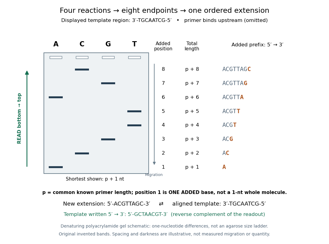
Read an original four-lane Sanger sequencing ladder from the shortest fragment upward to recover
. Invented ideal endpoints: A at extension positions 1 and 6; C at 2 and 8; G at 3 and 7; T at 4 and 5. Every fragment contains the same sequencing primer of length ; the shortest drawn band is nucleotides, not a one-nucleotide whole strand. The gel is a schematic of denaturing polyacrylamide gel electrophoresis; band spacing, widths and darkness are illustrative, with no measured migration, abundance or experimental photograph. The right panel shows the complete added prefix represented by each endpoint. Details.
Here is the full endpoint accounting. A terminal letter denotes an incorporated terminating nucleotide; all preceding letters of that extension were supplied by ordinary deoxynucleoside triphosphates.
The shortest fragments migrate farthest, placing position 1 at the bottom. Reading upward, the lane labels spell A, C, G, T, T, A, G, C: the new strand in its -to- direction. The adjacent T bands at positions 4 and 5 encode two separate additions. A single unresolved T patch would leave that count uncertain. In the A lane, the position-6 fragment passed position 1 using ordinary dATP and stopped at position 6 using ddATP; it does not skip the intervening nucleotides.
The common sequencing primer is an offset. For primer length , endpoint has length nucleotides. With an illustrative , the drawn fragments would contain 21 through 28 nucleotides, and adjacent endpoints still differ by one. Subtracting the common preserves their order because . This supplies a short justification for Sanger ladder reading: nested fragments share a start, length orders their endpoints, and lane membership supplies each endpoint's letter. A missing early band cannot be relabeled position 1 without independent evidence about the starting point.
To report the original template region, first complement the readout in aligned orientation:If the requested answer is that template written to , reverse the aligned template to obtain , the reverse complement of the readout. Reversing the readout alone would give CGATTGCA and would be wrong. Complementing without reversing gives the correct template letters in its displayed -to- direction, but not in the usual reporting convention. Specify the strand and its direction before transforming the answer.
Sagnac rotating-ring experiment 2026-10-18
In 1913 Georges Sagnac mounted a lamp, collimator, beam splitter, four mirrors and photographic plate on a horizontal rotating platform. The mirrors defined a closed polygon; the two beams traversed it in opposite senses. A slight beam splitter adjustment produced visible interference fringes. A motor brought the platform to steady rotation, and switching the lamp exposed the plate. Comparing opposite senses of rotation revealed a reversing displacement. Changing the beam splitter adjustment supplied a further check against optical deformation. The report compared measured and calculated displacements. Georges Sagnac interpreted this as evidence for a luminiferous aether; the relativistic derivation below reproduces the delay without that hypothesis.[ref]
Regarding the Proof for the Existence of a Luminiferous Ether Using a Rotating Inteferometer Experiment by Georges Sagnac. Georges Sagnac, 1913 second report, inspected in William Lonc's 2008 English translation, pp. 77–80, §§1–3: rotating apparatus, photographic procedure, reversal and deformation controls, comparison table, historical interpretation
The readout measures a relative wave phase, not two stopwatch readings separated by an optical transit time. Reversal isolates a contribution odd in angular velocity: if a signed interference fringe position is to leading order, then cancels the fixed offset . Changes of alignment or temperature correlated with reversal can survive this subtraction. Thus the experimental inference concerns a reproducible rotating-loop phase difference, with controls for disturbances; it is not by itself a unique test of an underlying propagation hypothesis.
Sagnac fringe shift worked example 2026-10-18
For a stationary rotating apparatus driven by a source with optical coherence and proper frequency , define . The source wave phase advances by between the emission times of the two contributions that meet at one readout spacetime event. Define the signed phase lag of the contribution and the corresponding displacement in units of one interference fringe byThe sign of a photographed spatial displacement also depends on the imposed fringe orientation; this definition fixes the theoretical sign through the delayed beam. In an equal-amplitude output, a representative light intensity is , where sets the chosen spatial interference fringe spacing . Moving by shifts the pattern by one fringe. A fixed output exactly at a bright or dark fringe has zero first-order intensity slope, so a known phase bias or a spatial fringe readout is useful for determining a small signed delay.
Choose a square of side , a rectangle by , and , with angular velocity parallel to the positive normal vectors. Both perimeters are , but the areas are and . Using , the leading predictions areThese are original model choices and predictions, not measured points. The square has times the response despite the equal path lengths. Reversing from to gives : the displacement magnitude between opposite rotations is twice the displacement magnitude from rest. Confusing these two comparisons introduces a factor-of-two error.
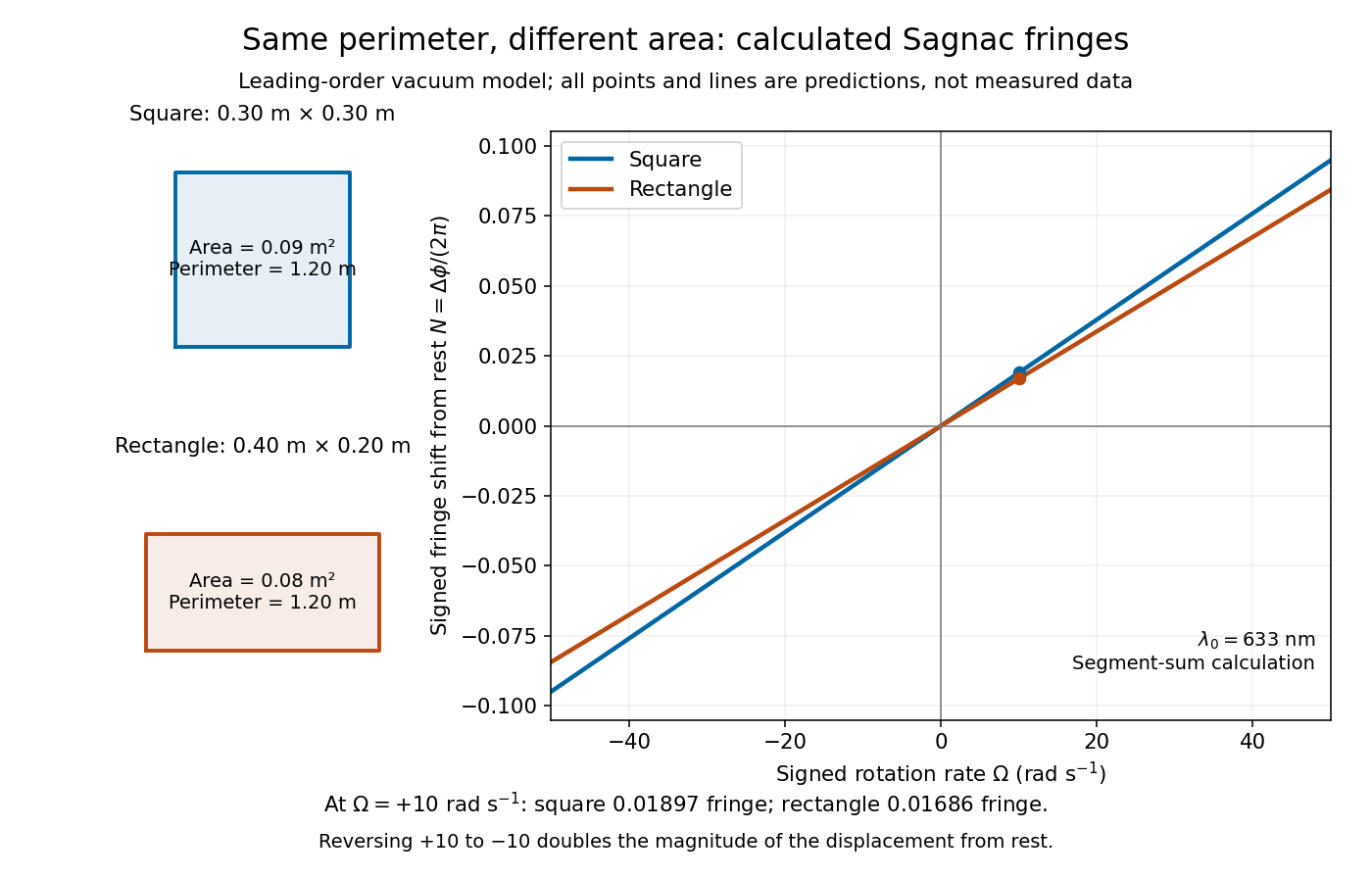
Independent path-segment calculation of the predicted fringe displacement for two equal-perimeter loops
. The generator sums along each straight segment, rather than inserting the enclosed area into the answer. Both loops are oriented counterclockwise. Lines and marked values are leading-order vacuum model predictions; no historical measurements are plotted. Details.
Sextic stabilization of a quartic saddle 2026-10-18
For every , the polynomial has exactly five stationary points: the origin and the four points with . Its gradient factors asIf a coordinate vanishes at a stationary point, both do. Otherwise put , to obtain and . Dividing gives and then .
At the origin, the Hessian matrix vanishes. Axis restrictions give , while diagonal restrictions give for small nonzero . Thus the origin is a degenerate saddle point of a scalar function. Its leading quartic term is nonpositive, showing why the sign of the first nonzero homogeneous term alone need not settle the problem when that term vanishes along some directions.
At each nonzero stationary point, the Hessian matrix has diagonal entries and off-diagonal entries . Its positive eigenvalues and prove strict local minima. They are also global minima of value : the arithmetic-geometric mean inequality gives , and the minimum of for is at . Equality requires .
There are unlisted articles, also show them or only show them.