
If the quadratic kinetic energy has a singular coefficient matrix, some generalized coordinates have no independent linearized inertia. The small oscillation equations can then contain algebraic constraints, and the number of finite normal mode frequencies can be smaller than the number of coordinates. One should use the polynomial without dividing by . Giving a nominally massless component a small mass can restore a high-frequency mode whose frequency diverges as that mass tends to zero.
Harmonic approximation Created 2026-10-18 Updated 2026-10-20
Near a stable equilibrium with and , the harmonic approximation truncates the Taylor series of the potential energy at quadratic order. With constant mass , Newton's second law then gives a harmonic oscillator with angular frequency . The approximation requires displacements small enough that the omitted terms are negligible; it does not describe a flat minimum where .
Giaever gap experiment 2026-10-18
Ivar Giaever's gap experiment used a metal–insulator–metal sandwich. His lecture describes evaporating aluminium onto glass, briefly exposing it to air to form an oxide barrier, then evaporating lead cross-strips. Cooling in liquid helium made the lead superconducting while the aluminium stayed normal in the measurements compared. A voltmeter and ammeter supplied the junction electric potential difference and electric current readouts. Thick oxides initially gave unmeasurably small electric currents; the thinner barrier made the measurement practical. Temperature comparisons and a subsequent controlled magnetic field test changed the current-voltage characteristic with the superconducting state. [ref]
The 1960 letter compares measurements at and . An applied parallel magnetic field of kept the lead normal; removing the magnetic field strongly suppressed the small-voltage electric current. Figure 2 divides the superconducting by the normal-state slope. The letter calls its gap estimates preliminary and notes a temperature-dependent broadened peak. It also flags a limitation of interpreting tunneling directly through the density of states; the ideal NIS calculation above states additional assumptions explicitly. [ref]
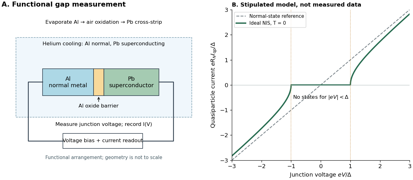

The central inference is that the barrier lets electric current interrogate available quasiparticle states. Suppression at small electric potential difference and the rise near the gap edge support a gapped spectrum; tracking the superconducting state helps distinguish that feature from an arbitrary nonlinear barrier. A leakage path through a metallic short, imperfect barrier, or an energy-dependent tunneling matrix element limits a literal density of states interpretation. The preparation and state controls therefore matter as much as seeing a nonlinear current-voltage characteristic.
Cooling schedule for simulated annealing 2026-10-18
A cooling schedule for simulated annealing specifies successive effective temperatures and how many proposals to attempt at each. For example, with , using the geometric sequence, can define stages of equal chosen length. Changing changes the transition matrix: if the state probability distribution is , then , which generally differs from . Time spent at one temperature must be compared with its mixing time before equilibrium intuition is justified.
In the five-state barrier example for simulated annealing, fixed gives a finite irreducible Markov chain, so is eventually visited with probability one. That unbounded-time statement gives no fixed finite deadline. Over any finite number of trials starting at , the probability of staying at throughout isEach factor is the rejection probability at . This is an explicit failure event even when every is positive: the best visited objective function value remains , above the global minimum value . More exploratory proposals can help cross a barrier; cooling before those moves occur can preserve a poor local minimum. Successful asymptotic schedules need additional analysis of the allowed moves and barriers.
Historically, Scott Kirkpatrick, Charles Daniel Gelatt Jr. and Mario P. Vecchi connected statistical mechanics with mathematical optimization in 1983. They adapted the Metropolis–Hastings algorithm to cooling searches with symmetric proposals and illustrated computer-design problems.[ref]
Optimization by Simulated Annealing by Scott Kirkpatrick and others. Printed pp. 672–673 and 675: Metropolis procedure, cooling schedule, logic partitioning
Fixed-temperature law of simulated annealing 2026-10-18
On a finite state space with finite objective function values, the fixed- target is a Boltzmann distribution:The partition function normalizes the weights but cancels from the Metropolis–Hastings acceptance probability. A short detailed balance proof explains the target. With symmetric and ,Summing over gives , so this is a stationary distribution. On a finite state space, a connected graph of positive symmetric proposals makes the accepted Markov chain an irreducible Markov chain. Convergence from any starting state additionally requires an aperiodic Markov chain; one positive self-transition suffices under irreducibility. Replacing by ensures this. For asymmetric , require connectivity through bidirectional proposals: one-way proposals are rejected.[ref]
In the five-state barrier example for simulated annealing, gives exact Boltzmann weights . Multiplying by givesFor the uphill edge, detailed balance is visible numerically:Thus the global minimum has the largest individual stationary probability, , but is far from certain at this positive . At the exact stationary distribution is .
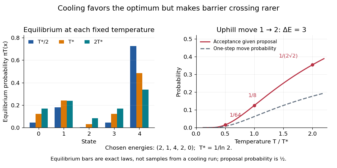
Lower temperature concentrates equilibrium weights while suppressing uphill acceptance
. Exact Boltzmann distributions for the chosen five-state objective function, and the uphill acceptance probability conditional on the proposal . The one-step transition probability is half that acceptance probability. The bars describe equilibrium at each fixed temperature, not the evolving probability distribution during cooling. Details.
For any finite , let be the set of global minima and the smallest objective function value. Cancelling from numerator and denominator shows that each nonminimal state's weight tends to zero as , while every state in has equal weight. Therefore tends to the uniform distribution on . This is a statement about a family of equilibrium probability distributions; it does not prove that a cooling Markov chain follows that family.
Consider the chosen finite minimization problemOnly adjacent integers are neighbors. At each interior state propose left or right with probability each; at an endpoint propose its sole neighbor with probability and itself with probability . This proposal distribution is symmetric, including at the endpoints. The local minimum at is relative to these allowed moves; is the unique global minimum.
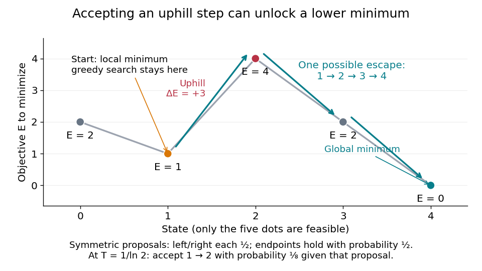

At , improving-only local search rejects both neighbors because and exceed . For simulated annealing, choose , using the natural logarithm. Conditional on proposing from , the acceptance probability isThe one-step transition probability is instead . Both subsequent rightward proposals are downhill, so the conditional probability of the precise next three states being , given and fixed , isThis is one possible escape route, not the probability of eventually reaching . Rejections, excursions toward , and repeated attempts give many other sample paths. The calculation establishes possibility, without claiming a general performance advantage from a selected sample path.
For comparison, halving makes the uphill acceptance probability ; doubling it makes that probability . Cooling makes it harder to leave this local minimum, even though the stationary distribution increasingly favors the global minimum. That tension is the central scheduling problem.
Radiative Sigma-to-Lambda transition 2026-10-18
The neutral Sigma baryon and Lambda baryon both have valence content , but different spin-isospin couplings. An electromagnetic transition changes those internal couplings without changing any quark flavour. In the simple ground-state quark model, the nonzero magnetic transition is associated with the up- and down-quark electromagnetic currents; the strange-quark spin operator alone cannot change the pair from spin one to spin zero. Four-momentum conservation gives photon energy in natural units.
Work by Sichen Shao 2026-10-18
The Fano factor compares count variance with its mean over a specified gate. For a stationary unidirectional stream with fixed charge , finite count second moments, and a generalized autocovariance with finite integral so that the long-gate limit exists,The zero-frequency relation concerns the continuous fluctuation spectrum, excluding the mean spectral line. It follows by writing as the double integral of the current autocovariance; for long , its leading term is . A finite-gate , a frequency-dependent ratio , and a factor inferred from one filtered variance are not interchangeable. The last is weighted by the instrument's .
Two original counting counterexamples show why electric charge discreteness is insufficient. In independent time slots, transfer one charge with probability in each slot: the binomial distribution gives mean , variance and Fano factor . A random common origin for the slots removes a preferred time origin; the long-gate factor remains . Alternatively, if independent Poisson process bursts each transfer exactly two charges, then gives and factor . Both count individual charges; only the first model allows at most one per slot, and the second groups them in pairs.
Consequently is a reference for independent unidirectional arrivals, not a universal noise law for all electrical conductors. Correlations, charge multiplication, and bidirectional transfer require a more specific model. For example, independent opposite streams with positive current magnitudes and have net mean but one-sided fluctuation spectrum . Using would miss their fluctuations when the net current is small. At thermal equilibrium, the full transport model must also respect thermal electrical noise; adding unrelated phenomenological formulas can double count the same underlying transfers.
Shot noise photocurrent measurement 2026-10-18
MIT's guide uses an illuminated vacuum photodiode, with collecting anode positive relative to the emitting cathode. A transimpedance amplifier gives ; a multimeter reads its mean. The fluctuation path rejects below , adds roughly tenfold voltage gain, then nominal hundredfold preamplification and a – band-pass filter; the readout measures root mean square voltage. With diode bias off, a sinusoid at the test port calibrates . Restore bias, retain gain settings, vary lamp brightness, and repeat both readings. The guide warns about overload; it supplies a procedure, not measured results.[ref]
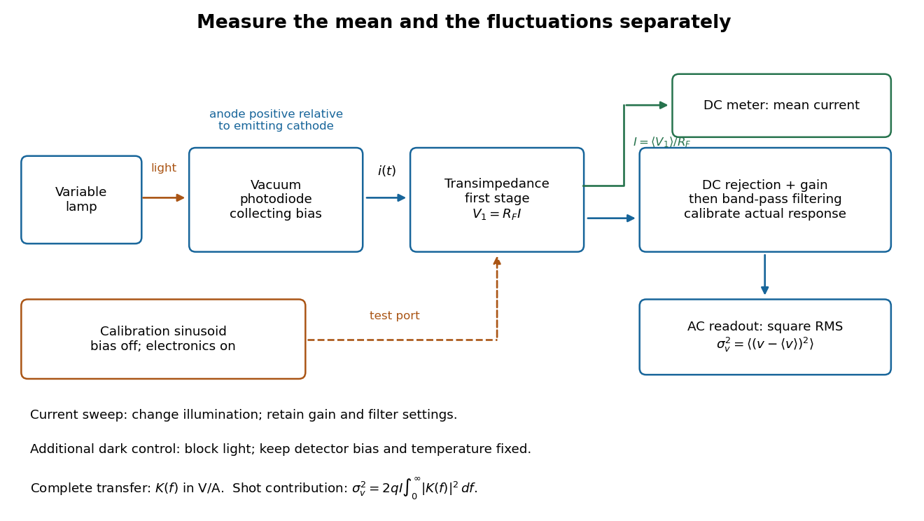
Functional photocurrent measurement: separate mean-current, fluctuation and calibration paths
. Original functional diagram organizing the laboratory's measurement roles; it is not a component-level circuit reproduction. includes current-to-voltage conversion and the complete fluctuation path. The dark comparison below is an additional control. Details.
The inference can be expressed without relying on nominal passband edges. Let denote the calibrated voltage transfer after the conversion, so and define . Under independent arrivals and an unchanged additive background,The slope of voltage variance against mean electric current can therefore estimate . A free intercept accounts for a constant background; forcing the line through zero generally biases the slope. The root mean square readings must have their mean removed and then be squared. Subtracting two root mean square amplitudes does not subtract independent variances. Estimate the variance from successive records; averaging the waveforms first would suppress the fluctuation being measured.
Additional controls sharpen this interpretation. Block the light with detector bias, temperature, and gain unchanged; this preserves dark current and electronics while removing photocurrent. Repeat this dark comparison between illumination settings to check drift. If independent dark arrivals have mean magnitude and illuminated arrivals add , their spectra add: . Subtracting the unchanged dark variance isolates . This subtraction model assumes unchanged transfers and independence; switching off bias for gain calibration is a different control and need not preserve the dark background.
Vary measured rather than assuming lamp knob position is proportional to photocurrent. Check collection versus bias to identify a range where incomplete collection is negligible; a space charge limited tube can correlate transfers. Verify that the transimpedance amplifier remains linear and that its frequency response is unchanged over the illumination range. Changing signal bandwidth should change the excess variance through ; compare inferred input spectra in several bands. Correlated fluctuations of the light source can add a contribution scaling approximately as , while an electronics floor can hide the linear term at small electric currents. A fitted line over a short range alone does not establish independent transfers.
The gain calibration must include the same detector-to-readout path used for noise, or explicitly supply any omitted transfer. Detector capacitance, finite collection time, amplifier voltage and current noise, thermal electrical noise, pickup, clipping, and finite recording precision limit the inference. Current-dependent electrical impedance or heating can make a background current-dependent too. Since contains squared gain, a small fractional error in gain produces approximately twice that fractional error in the predicted variance scale. Knowing a nominal gain and two cutoff settings is insufficient.
Shot noise worked example Created 2026-10-18 Updated 2026-10-20
For an original model, set , , , , and the exponential low-pass filter's . Assume an ideal detector without charge multiplication and omit all additive noise for this calculation. ThenDoubling doubles the voltage variance and multiplies its standard deviation by . Halving also doubles the variance, provided the detector remains approximately white throughout the enlarged passband. Using in place of underestimates the variance by the factor . These are calculated predictions, not measured values or settings claimed for the laboratory below.
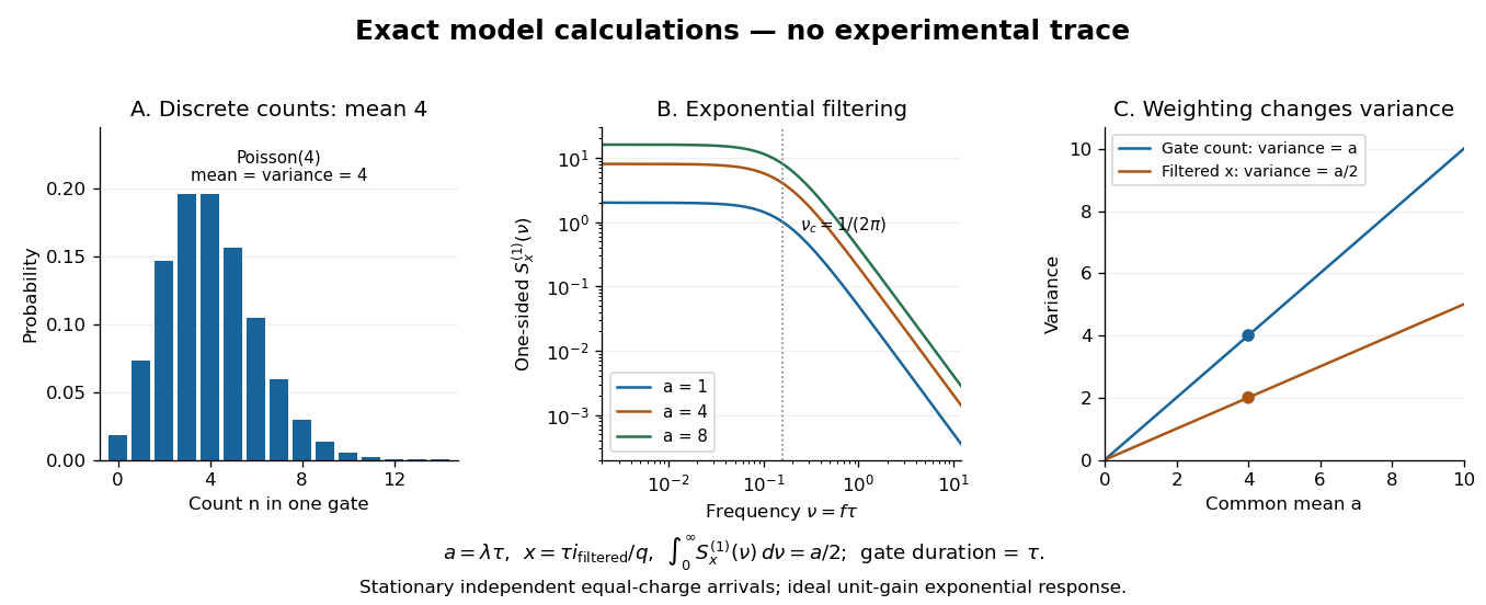

To read the dimensionless figure, set and , with frequency in cycles per unit . A gate of duration has count mean and variance . The continuously filtered instead hasThe count and the filtered electric current are different observables. The factor comes from the exponential weighting, not from non-Poisson arrivals. The dimensionless count illustration is a separate choice of rate; it does not assert that the example has only four electrons per .
Filtered shot noise 2026-10-18
Let be the complete current-to-voltage frequency response from detector input to readout, in . For a real stable linear time-invariant system, the shot contribution to the output voltage variance isIf with feedback electrical resistance , a reference voltage gain , and dimensionless normalized frequency response , thenThis is the effective noise bandwidth for unit reference magnitude. The transimpedance amplifier factor converts electric current to voltage; multiplies voltage. Neither is an additional noise source merely because it amplifies an existing fluctuation. In contrast, a real amplifier adds input voltage noise and input current noise, and its feedback resistor contributes thermal electrical noise. Those terms need their own transfers to the output. In particular, input voltage noise generally has a different transfer from an injected detector electric current. Simply multiplying every input specification by is incorrect.
For a unit-gain exponential low-pass filter, with time constant ,The cutoff frequency is not . An independent time-domain derivation sums independent event contributions to giveThe same reasoning for a rectangular averaging gate has on and zero elsewhere, hence effective noise bandwidth and variance , agreeing with the shot noise counting model. Equal numerical durations do not make these two different linear filters equivalent.
Shot noise spectral convention 2026-10-18
Write an ideal point-transfer model using the Dirac delta function:For this arrival stream with independent increments, distinct arrivals contribute the product of the means, which cancels when centering. The same-arrival term leaves the autocovarianceIts Fourier transform gives the two-sided power spectral density, while folding negative frequencies onto positive ones gives the one-sided convention:These spectra describe , excluding the spectral line from the mean direct current. The amplitude spectral density is in ; it is not a root mean square electric current until a measurement signal bandwidth is specified. Approximate white noise requires frequencies low enough that the single-transfer pulse shape and any correlations can be neglected. Neither the ideal impulses nor a flat spectrum extending to infinity describe a real detector at every timescale.
All spectra above are per hertz, with in cycles per second. One possible angular frequency convention defines a density integrated using alone. Since , it hasAnother common convention keeps the numerical density but integrates it with . State the integration measure as well as whether a spectrum is one-sided: a change of variable and a folding of signs are separate operations.
Shot noise counting model Created 2026-10-18 Updated 2026-10-20
Let be the magnitude of each transferred electric charge, and let arrivals form a Homogeneous Poisson process of rate . Extend the stream over past and future times when considering stationary filtering. For electrons, , the elementary charge. Choose the positive electric current direction to follow these transfers, so is its mean magnitude. If counts arrivals in a gate of duration , thenThe gate's transferred electric charge is , and its average electric current is . Scaling the expected value and variance givesMore arrivals increase the absolute fluctuation but decrease its size relative to the mean. For an original count example with , the mean count and its variance are both , the standard deviation is , and the relative standard deviation is . The probability of no transfer is ; the probability of four is . A constant arrival rate does not prescribe four arrivals in every gate.
These are fluctuations of a time average, not the variance of an ideal instantaneous electric current. A model of point transfers has arbitrarily sharp impulses; it acquires a finite measured variance only after specifying a gate or linear filter. Actual collection pulses have finite duration and electrical circuits have finite response times.
Cubic series reversion 2026-10-18
Suppose with . Substitute and compare coefficients. The three equations are , , and . Solving them proves the title formula. This is series reversion for a local inverse function; analyticity guarantees a convergent inverse series sufficiently near the origin.
Direct comparison test Created 2026-10-18 Updated 2026-10-25
If eventually and converges, then converges. The nondecreasing partial sums of the nonnegative are bounded above by a finite initial contribution plus the sum of ; bounded monotone sequence theorem proves the claim. Consequently with summable proves absolute convergence of . Finite changes to initial terms do not affect convergence.
Decay of a Fourier mode in a third-order spatial evolution equation Created 2026-10-18 Updated 2026-10-25
A separated Fourier mode with initial value at obeys and . Its amplitude decays for precisely when . The zero mode stays constant and negative modes grow. Thus a decay requirement on a half-space imposes a sign condition on the real wave number; a formal separated expression alone does not establish compatibility of both boundary conditions.
Concentration blob Created 2026-10-18 Updated 2026-10-20
A region of size containing a typical correlated chain segment whose internal monomer concentration matches the bulk concentration. If it contains statistical units with isolated size law and unit volume , concentration matching gives . Eliminating gives . Numerical prefactors and distinctions among scattering, osmotic and geometric correlation lengths require additional definitions.
Laser diode Created 2026-10-18 Updated 2026-11-05
A laser diode is an electrically injected semiconductor laser. Forward biasing supplies electrons and electron holes to an active region, where radiative recombination can amplify a compatible optical mode by stimulated emission.
Reflecting facets or other cavity structures provide feedback. Below the laser threshold, emission is dominated by spontaneous processes; above it, stimulated emission into resonator modes becomes important. A light-emitting diode can also use carrier recombination but does not require this feedback-and-gain threshold. Output power, emitted spectrum and terminal current-voltage characteristic together characterize the device more fully than brightness alone.
MOS inversion threshold Created 2026-10-18 Updated 2026-10-20
For an ideal MOSFET with a nondegenerate p-type semiconductor of acceptor density , define , where is the intrinsic carrier concentration. A positive surface electric potential lowers the local conduction band and valence band by . The surface electron density is . Equality gives the conventional onset of strong inversion at . The earlier crossover occurs at . Neither condition requires the Fermi level to enter the conduction band.
There are unlisted articles, also show them or only show them.