
Work by T. Bressani 2026-10-18
Work by Susanne Kiewitz 2026-10-18
Band bending Created 2026-10-18 Updated 2026-10-20
Spatial variation of the valence band and conduction band edges associated with a varying electric potential. Near a semiconductor boundary it can deplete mobile charge carriers or create a semiconductor inversion layer.
Institutional appendix; no separate personal byline. Defines stopping powers, CSDA and projected ranges, and detour factor.
High-speed charge and isotope scaling of electronic stopping Created 2026-10-18 Updated 2026-10-20
For a fast ion traversing a fixed material thickness with only a small fractional energy loss, the dipole excitation probability per atomic encounter scales as at fixed impact parameter. Summing transferred excitation energies and integrating the encounter measure gives the leading electronic stopping power scaling, with slower logarithmic dependence from the allowed excitation energies and impact-parameter range.
At fixed ion kinetic energy , a heavier isotope is slower, so the leading loss scales as . At fixed velocity, isotopes of the same element instead have approximately the same electronic loss; plotting against energy per nucleon removes the leading isotope mass dependence. The charge should be the effective projectile charge if its bound electrons screen the nucleus. At lower speeds, excitation thresholds, slow-passage suppression, charge exchange and nuclear energy transfer invalidate a simple extrapolation of the high-speed law.
Work by Stig Lundqvist 2026-10-18
Work by Stiftung Werner-von-Siemens-Ring 2026-10-18
Work by Steven Rolston 2026-10-18
Quantum fluid Created 2026-10-18 Updated 2026-11-05
A quantum fluid is a fluid whose collective behavior requires quantum mechanics, particularly when the thermal de Broglie wavelength becomes comparable with particle spacing. Exchange statistics and interactions then affect the state in ways that a dilute classical particle model cannot capture. Low temperature favors this regime, but temperature alone is insufficient without a density and particle-mass scale.
Superfluid helium-4, degenerate fermionic matter described by a Fermi liquid, and dilute ultracold atomic gases provide different realizations. A quantum fluid need not be a superfluid, and quantum degeneracy does not by itself remove dissipation. Measurements of heat capacity, collective waves and response to flow distinguish the relevant states. The useful organizing question is which low-energy excitations carry energy, momentum and conserved particle number, rather than whether individual particles merely have small kinetic energies.
Non-Fermi liquid Created 2026-10-18 Updated 2026-11-05
A non-Fermi liquid is an interacting fermionic state whose low-energy behavior is not described by the long-lived quasiparticles of a Fermi liquid. In the conventional Fermi liquid picture, excitations close enough to the Fermi surface become sharp compared with their excitation energy. If that organizing principle fails, extending the same quasiparticle approximation toward zero energy can give the wrong response.
The term describes a failure of one framework, rather than one unique replacement theory. A one-dimensional Luttinger liquid provides a controlled example: its long-wavelength excitations are collective density modes, and its correlation functions need not have the free-fermion form. An anomalous finite-temperature transport curve alone does not establish a particular zero-temperature non-Fermi liquid. Spectral and thermodynamic measurements must be interpreted alongside the relevant dimensionality, interactions and accessible energy range.
Energy landscape 2026-10-18
An energy landscape assigns an energy to each possible state and describes its variation between neighbouring states. Its local minima and intervening energy barriers help distinguish favourable states from states that a specified dynamics can reach quickly. In a Hopfield network, the assigned energy is an objective function and need not be a conserved physical quantity.
Thermal activation Created 2026-10-18 Updated 2026-11-05
Thermal activation is barrier crossing enabled by thermal fluctuations. A system can remain for a long time near a local minimum of an energy landscape, then receive a fluctuation large enough to cross an energy barrier. Its most probable state and its waiting time for escape are therefore different questions.
In a simple high-barrier regime, the escape rate is approximated by , an Arrhenius equation. The barrier controls the strong temperature dependence, while the prefactor depends on dynamics near the initial state and transition region. Plotting against tests the exponential model: a constant prefactor gives slope . Interpreting a slope still requires care if several escape paths compete or the prefactor varies with temperature. A large barrier can delay approach to thermal equilibrium even when the final equilibrium state is known.
Linear response theory Created 2026-10-18 Updated 2026-11-05
Linear response theory approximates a small change in an observable by a linear function of an applied perturbation around a specified reference state. A weak force can produce a proportional displacement, and a weak applied magnetic field can produce proportional magnetization. The response coefficient depends on the material and state; linearity is an approximation to test by changing the drive size.
For a causal time-dependent response, writeThe kernel describes the delayed effect of the perturbation . A sinusoidal input probes the frequency-dependent response: its in-phase part and out-of-phase part determine the response magnitude and phase lag. Causality links the real and imaginary parts through Kramers-Kronig relations under the appropriate convergence assumptions. Comparing the response at several small drive sizes tests linearity; a linear-looking response at one size alone cannot establish the range of validity.
Hard sphere 2026-10-18
A hard sphere has an impenetrable core and otherwise no pair interaction. Two identical spheres of diameter cannot have centre separation below . Even without attractive potential energy, crowding can produce fluid–crystal coexistence because available configuration space and entropy differ between the phases.
Lattice gas Created 2026-10-18 Updated 2026-10-20
A lattice gas describes particle positions by occupations of fixed cells. In the single-occupancy model, and . Its grand canonical partition function sums configurations with weight . Discretizing a classical position integral into cells of volume gives , with thermal de Broglie wavelength .
Lesson in STAT 414: Introduction to Probability Theory at Pennsylvania State University. No individual author byline or separate lesson date is established. The institutional search-indexed text was inspected; the direct page fetch failed.
Official lesson: online.stat.psu.edu/stat414/Lesson11
Linear Stark effect in the first excited hydrogen eigenspace Created 2026-10-18 Updated 2026-10-20
Consider a fixed proton and one electron, omitting spin, fine structure and the Lamb shift. Let be the elementary charge, the Bohr radius in this fixed-nucleus model, and . Because the electron's electric dipole moment is , its electric-dipole interaction isThe first excited hydrogen eigenspace has a common unperturbed energy eigenvalue . Write and in the hydrogen energy eigenbasis. The electric-dipole selection rules for hydrogen leave only the coupling within this eigenspace. Each diagonal matrix element vanishes by parity, but that does not make the entire perturbation vanish. Degenerate perturbation theory requires its eigenvalues in the whole eigenspace. With the usual real wavefunction phases the off-diagonal position matrix element is .[ref]
Linear Stark Effect. Quantum Mechanics by Richard Fitzpatrick; Fitzpatrick, Linear Stark Effect, equations (7.82)–(7.86)
The factor three can be checked directly. Set and use normalized radial wavefunctions and spherical harmonics:The angular integral is . Including and the radial volume factor then givesReversing the quantum phase of reverses this sign, with no change to the predicted energy eigenvalues.
Thus the nontrivial two-dimensional block and its determinant equation areConsequently, for the displayed sign convention,The two remaining energy eigenstates have zero first-order shifts. The slopes correspond to opposite electric dipole moments, and . The electric field selects combinations of opposite parity that already have these dipole expectations at leading order. This is why applying first-order nondegenerate perturbation theory separately to and , and obtaining two zero diagonal entries, misses the splitting.
The approximation requires small compared with the separation to other principal quantum numbers. For real hydrogen atoms, it also requires the relevant electric-dipole interaction to dominate the small splittings omitted here, including the Lamb shift. At sufficiently small electric fields a pre-existing nonzero – separation must be retained before taking the limit. A simple two-state illustration with unperturbed separation has shifts relative to its meanFor , the lower branch moves by relative to its zero-field value. At the splitting is linear. This interpolation explains the importance of the hydrogen energy-level degeneracy; it is not a complete model of the fine structure multiplet.
Stark canal-ray experiment 2026-10-18
In 1913 Johannes Stark reported that an applied electric field resolved the hydrogen and spectral lines into five components at his instrument's spectral resolving power, viewed perpendicular to the electric field. Three inner components had polarization of an electromagnetic wave perpendicular to the electric field; two outer components had it parallel.[ref]
Observation of the Separation of Spectral Lines by an Electric Field by Johannes Stark. Stark, Nature 92 (1913), p. 401, two opening paragraphs; issue dated 4 December
In his lecture of 3 June 1920 for the 1919 prize, Johannes Stark describes canal rays emerging through a perforated cathode into the electric field between it and a supplementary electrode. A spectrograph recorded the emitted light. His earlier Doppler effect comparison used a collimator perpendicular to the beam and then along approaching rays. Later beam/electric field reversal changed component intensities.[ref]
Structural and Spectral Changes of Chemical Atoms by Johannes Stark. Nobel Lectures, Physics 1901–1921; Stark, Structural and spectral changes of chemical atoms, printed pp. 430, 433–435; lecture date p. 427
The historical account distinguishes observation perpendicular to the electric field, with five resolved components, from observation parallel to it, with three. These are viewing directions, distinct from the direction of the polarization of an electromagnetic wave.[ref]
The Discovery of the Stark Effect and Its Early Theoretical Explanations by A. J. Kox. Kox, The discovery of the Stark effect and its early theoretical explanations, §2 Johannes Stark, paragraph following Figure 2
The experimental distinctions matter. Changing the viewing direction tests a Doppler effect contribution; changing the applied electric field tests the Stark effect; analyzing polarization of an electromagnetic wave separates components that may overlap in an unpolarized record. A comparison with the unperturbed spectral line fixes the origin of a displacement. These are different controls, and the earlier Doppler effect comparison should not be described as a field-off control of the later discovery. A spectrograph's finite spectral resolving power can merge several components into one. In particular, a count of visible spectral lines does not by itself count all energy eigenstates.
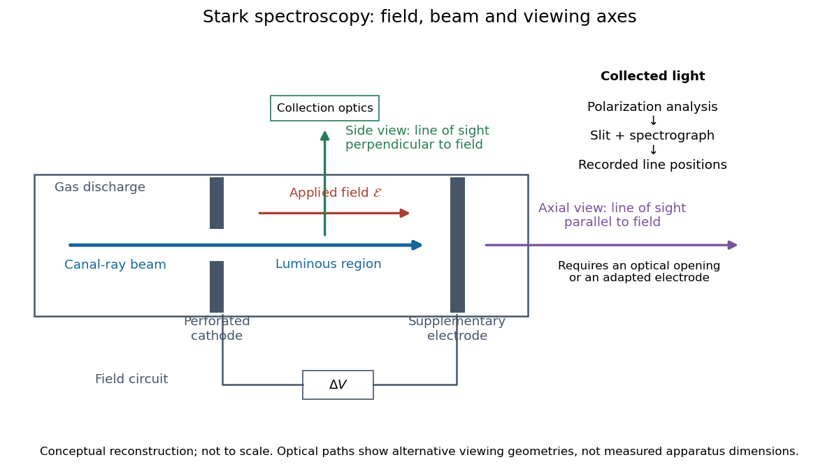
Stark spectroscopy: field, beam and viewing axes
. Original conceptual reconstruction of the canal ray source and two alternative viewing geometries. No dimensions, electric field strengths or measured wavelengths are specified. The axial optical path requires an opening or adapted electrode; it is not a ray passing through the solid electrode drawn here. Details.
For a modern idealization of the gap, an electric potential difference over separation gives only if edge effects and the charge density in the gas are negligible. This is a calibration model, not a historical value assigned to Stark's apparatus. Similarly, a canal ray beam need not be a pure beam of neutral excited hydrogen atoms; the quantum mechanics model below isolates one neutral hydrogen atom from the source's preparation and collision processes.
Quadratic Stark effect Created 2026-10-18 Updated 2026-10-20
The quadratic Stark effect is an energy level shift whose leading term is quadratic in an applied electric field. For a nondegenerate energy eigenstate of definite parity, the diagonal matrix element of an odd electric-dipole perturbation vanishes. Second-order nondegenerate perturbation theory givesEvery term is negative for the ground state. If field reversal is implemented by the parity operator, an analytic nondegenerate energy branch is even in the field. This symmetry explains the absence of odd powers; it does not apply without qualification to a degeneracy split linearly by the field.
There are unlisted articles, also show them or only show them.