
Topological atlas Created 2026-10-14 Updated 2026-10-31
A topological atlas is a family of coordinate charts whose domains form an open cover of a topological manifold. Each point must belong to at least one chart domain; no individual domain needs to cover the entire topological manifold. On overlaps, topological transition maps describe the same points in two coordinate systems.
Work by Thomas W. Burns 2026-10-14
Work by Thomas Little Heath Created 2026-10-14 Updated 2026-10-25
Thermodynamic process 2026-10-14
A thermodynamic process changes a thermodynamic system between states. A quasistatic process supplies equilibrium intermediate states and therefore a path on equilibrium coordinates. An irreversible thermodynamic process can have equilibrium endpoints while lacking a uniform intermediate temperature or pressure. Endpoint values still determine changes in a state function; computing heat and work requires the actual interaction history.
Thermodynamic state 2026-10-14
An equilibrium thermodynamic state specifies sufficient independent macroscopic properties, together with material identity and constraints, to determine the other equilibrium properties. For a uniform fixed-composition ideal gas, its amount of substance, temperature and volume determine its pressure through the ideal gas law. These properties specify a state, without specifying a thermodynamic process that prepared it.[ref]
International Temperature Scale of 1990 Created 2026-10-14 Updated 2026-10-18
The International Temperature Scale of 1990 is a practical scale for reproducible temperature measurements. Its assigned reference points and interpolation procedures approximate thermodynamic temperature. A calibrated standard platinum resistance thermometer transfers this scale over specified intervals; it does not define the modern kelvin.[ref]
The International System of Units (SI), ninth edition, SI Brochure. §2.3.1: practical temperature scales, ITS-90, and thermodynamic temperature
Work by T. Lee 2026-10-14
Polarization-gradient cooling Created 2026-10-14 Updated 2026-10-18
Polarization-gradient cooling uses spatial variation in electromagnetic polarization together with optical pumping between internal quantum states to cool moving chemical atoms.
Jean Dalibard and Claude Cohen-Tannoudji distinguish cooling by changing elliptical polarization from cooling by rotating linear polarization. The hill picture below concerns the former.[ref]
Work by Steffen Rudtsch 2026-10-14
The UCSB demonstration uses an aluminum cylinder turned by a crank, with a wrapped rope supporting a hanging mass. An embedded electrical thermometer connects through sliding contacts to an electrical resistance meter; a supplied electrical resistance–temperature table or fitted equation converts the readout. A counter records turns. Record the initial temperature, crank steadily, then stop and convert the minimum recorded electrical resistance to the final temperature.[ref]
52.33 -- Mechanical equivalent of heat. UCSB Physics Lecture Demonstrations; UCSB demonstration 52.33, opening apparatus paragraphs and “Operating the demonstration”: cylinder, rope, turn counter and resistance calibration
The proposed control is to start below room temperature and finish comparably above it, approximately balancing incoming and outgoing environmental heat. Neglected accessory heat capacities and rough temperature estimates limit accuracy. The mechanical input and thermal response test an energy balance; warming alone does not establish quantitative equivalence.[ref]
52.33 -- Mechanical equivalent of heat. UCSB Physics Lecture Demonstrations; UCSB demonstration 52.33, final operating paragraphs: symmetric temperature preparation, environmental heat exchange and omitted apparatus capacities
This is a modern companion to Joule's paddle-wheel experiment, with a different apparatus. Choose the cylinder as the closed system. When endpoint bulk mechanical energy changes are negligible, a model for its thermal storage iswhere is its participating heat capacity, approximately constant over the run, and is signed environmental heat. The cylinder is not an isolated system, since mechanical work enters. The temperature rise estimates a change in internal energy, rather than an amount of externally supplied heat. This boundary distinction connects a measured thermal response to the same stored quantity used in two reversible ideal-gas paths between the same states.
Take a closed system consisting of one mole of a classical monatomic gas, idealized as an ideal gas with constant heat capacity at constant volume . Stipulate amount of substance and molar gas constant for this calculation. Set initial temperature and volume , and define and . The specified equilibrium endpoints areThus has volume , temperature and pressure . The fixed material inventory and ideal gas law make these complete endpoint specifications for this model. All numbers below are calculated values, rather than measurements of a particular gas.
Use a frictionless piston, ignore bulk mechanical energy changes, and allow only pressure-volume work. Each step is the limit of a reversible thermodynamic process: adjust loads by infinitesimal pressure differences, and supply heat through infinitesimal temperature differences. Heating with changing temperature requires a succession of matching thermal reservoirs; contact with a single hotter heat bath would give an irreversible finite difference. On a fixed-volume leg the piston is locked. These assumptions justify using the actual equilibrium path's pressure inAn endpoint chord is not the path; substituting a guessed straight line would compute a different thermodynamic process.[ref]
Thermodynamics and Propulsion. Thermodynamics and Propulsion, §1.3.3, Figures 1.10–1.11: external pressure versus equilibrium gas pressure in boundary work
The upper route heats at fixed volume from to , then undergoes isothermal expansion at to . The lower route undergoes isothermal expansion at from to , then heats at fixed volume to . The tuples use the same ordering as the endpoints. Vertical legs do zero expansion work, and the two curved legs have different pressures at every shared intermediate volume.
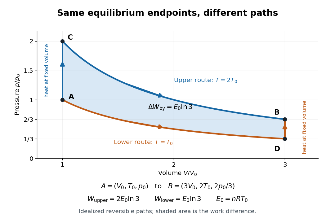
Two reversible ideal gas paths connect the same equilibrium endpoints
. Original idealized pressure-volume diagram. The upper route is and the lower route is ; the shaded gap is the difference in work, not an experimental uncertainty. Both are reversible thermodynamic processes under the stated piston and thermal reservoir assumptions. Details.
The internal energy of an ideal gas gives the same endpoint difference for both routes:On either fixed-volume heating leg, and . On each isothermal expansion, , so the first law of thermodynamics gives . The ideal gas law and the integral of then giveHere is the natural logarithm. Rounded to , the upper route has and the lower route has . Subtracting separately rounded entries can differ by ; the unrounded balances are exact in the stipulated model.
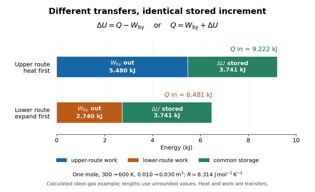

The shaded area between the curves explains the entire difference:Following the upper route forward and the lower route backward makes a thermodynamic cycle with this positive net work and matching net heat. Its internal energy change is zero. The two open routes themselves are reversible, so their different work outputs should not be mistaken for a loss caused by entropy production: they receive different heat transfers at different temperatures.
Two other state functions provide independent endpoint checks. With enthalpy in this model,To obtain the entropy change along either route, integrate on its heating leg, giving , and on its isothermal expansion, giving . Reordering the legs changes their heat totals but leaves the sum of their entropy changes unchanged. In particular, neither route's total divided by its final temperature equals , and neither total equals : both routes include an isothermal expansion, rather than a single fixed-pressure heating step.
Mixed spreadsheet reference 2026-10-14
A mixed spreadsheet reference fixes exactly one coordinate.
$A2 fixes column A and lets the row follow the copy; B$1 fixes row 1 and lets the column follow the copy. Put in A2:A4 and in B1:D1. Store =$A2*B$1 in B2, then fill the rectangle B2:D4. The colon denotes the inclusive rectangular range between the named corner spreadsheet cells. Each spreadsheet formula reads its row's factor from column A and its column's factor from row 1, producing a multiplication table.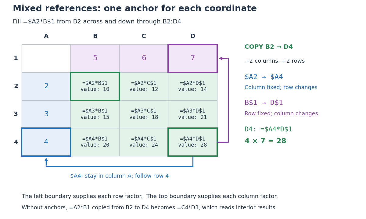
Original multiplication table showing how two mixed spreadsheet references anchor the column and row independently during two-dimensional copying
. Details. 
Copying from
B2 to D4 moves two columns right and two rows down. The mixed spreadsheet references become $A4 and D$1, so D4 contains =$A4*D$1 and has value . For comparison, under that same displacement A2 becomes C4, $A$2 remains $A$2, $A2 becomes $A4, and A$2 becomes C$2. These four cases express the independent choice for each coordinate. Microsoft's official table demonstrates the same four possibilities for a two-row, two-column copy. [ref]Switch between relative, absolute, and mixed references, Microsoft Support. Switch between relative, absolute, and mixed references: final four-row table, absolute column/row, relative column/absolute row, absolute column/relative row, and relative column/row
The filled rows have values , , and . The multiplication table works because the left factor moves only vertically and the top factor moves only horizontally. Without the anchors, copying
=A2*B1 from B2 to D4 would give =C4*D3, reading interior results rather than the intended boundary inputs.// Target: computer-science.bigb
Absolute spreadsheet reference 2026-10-14
An absolute spreadsheet reference, such as
$F$1, fixes both coordinates when its spreadsheet formula is copied. In the spreadsheet tabular model, every copied total reads the same tax rate. Absolute addressing retains the spreadsheet cell reference, not the value: changing the input in F1 changes the computed totals even though the references remain $F$1. Relative spreadsheet reference 2026-10-14
A relative spreadsheet reference, such as
A2, allows both coordinates to change when its spreadsheet formula is copied. From C2, A2 means two columns left, in the same row. Copy =A2*B2 from C2 to C4: the displacement is zero columns and two rows, so it becomes =A4*B4. The row number changes to retain the same positional relationship to the spreadsheet formula. Interspike interval Created 2026-10-14 Updated 2026-11-05
An interspike interval is the elapsed time between consecutive action potentials in a spike train. Its probability distribution and dependence on previous activity can reveal a neuronal refractory period even when the average firing rate is unchanged.
Germination Created 2026-10-14 Updated 2026-11-05
Seed germination is renewed plant embryo activity and growth. Many germination assays score completion as radicle emergence, before seedling establishment. Seed imbibition precedes that endpoint; swelling alone is insufficient.[ref]
Seed dormancy and the control of germination by William E. Finch-Savage and Gerhard Leubner-Metzger. Seed dormancy and the control of germination, §II.1, p. 502: water uptake, embryo expansion and radicle protrusion
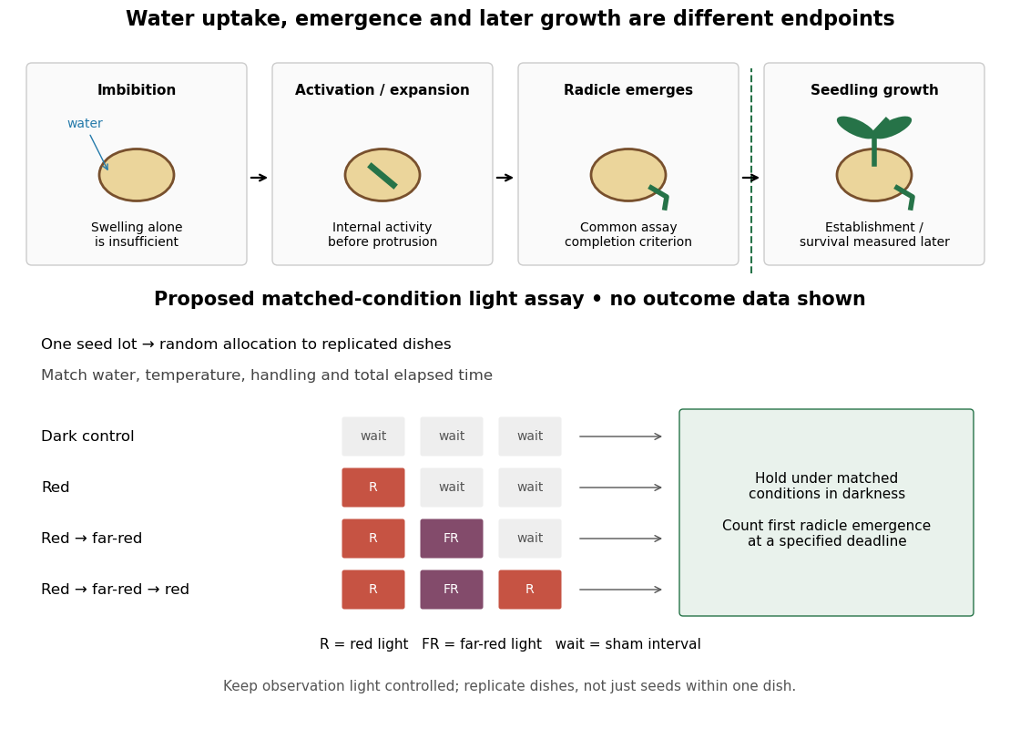

Water, molecular oxygen and suitable temperature support germination; light sensitivity depends on the species and seed state. Neither illumination nor one particular temperature is universally required. Seed dormancy connects germination timing to ecology by delaying seedling establishment.[ref]
Seed dormancy and the control of germination by William E. Finch-Savage and Gerhard Leubner-Metzger. Seed dormancy and the control of germination, Summary and §II.1–2, pp. 501–502: environmental requirements and timing
The distinction matters when comparing propagation experiments: a treatment that increases radicle emergence need not improve later seedling survival. Define the endpoint before comparing treatments, then measure the later outcome separately.
Seedling 2026-10-14
A young plant developing after germination. Early growth can use a seed food reserve before leaves support photosynthesis.[ref]
Biology 2e by Mary Ann Clark and others. Biology 2e, §32.2 Development of the Seed: reliance on cotyledon reserves before leaf photosynthesis
Endosperm 2026-10-14
A nutritive plant tissue distinct from the plant embryo; it may remain in the mature seed or be depleted during development.[ref]
Biology 2e by Mary Ann Clark and others. Biology 2e, §32.2 Development of the Seed: endospermic and non-endospermic seeds
Seed food reserve 2026-10-14
Stored material supporting early seedling growth, located in cotyledons, endosperm or other plant tissues depending on the plant.
Seed coat 2026-10-14
The protective covering of a seed, formed from maternal plant tissues surrounding the developing plant embryo.
There are unlisted articles, also show them or only show them.