
PCR extension Created 2026-10-14 Updated 2026-10-18
PCR extension is template-directed construction of DNA from an annealed PCR primer by a DNA polymerase. Incoming deoxynucleoside triphosphates supply the new nucleotides. Each addition lengthens the growing strand at its end, so the product grows while the template is read . The direction refers to the nucleic acid backbone, not to left or right on a page.[ref]
Principles of PCR by Thermo Fisher Scientific. Description, final paragraph: extension of annealed primers by dNTP incorporation
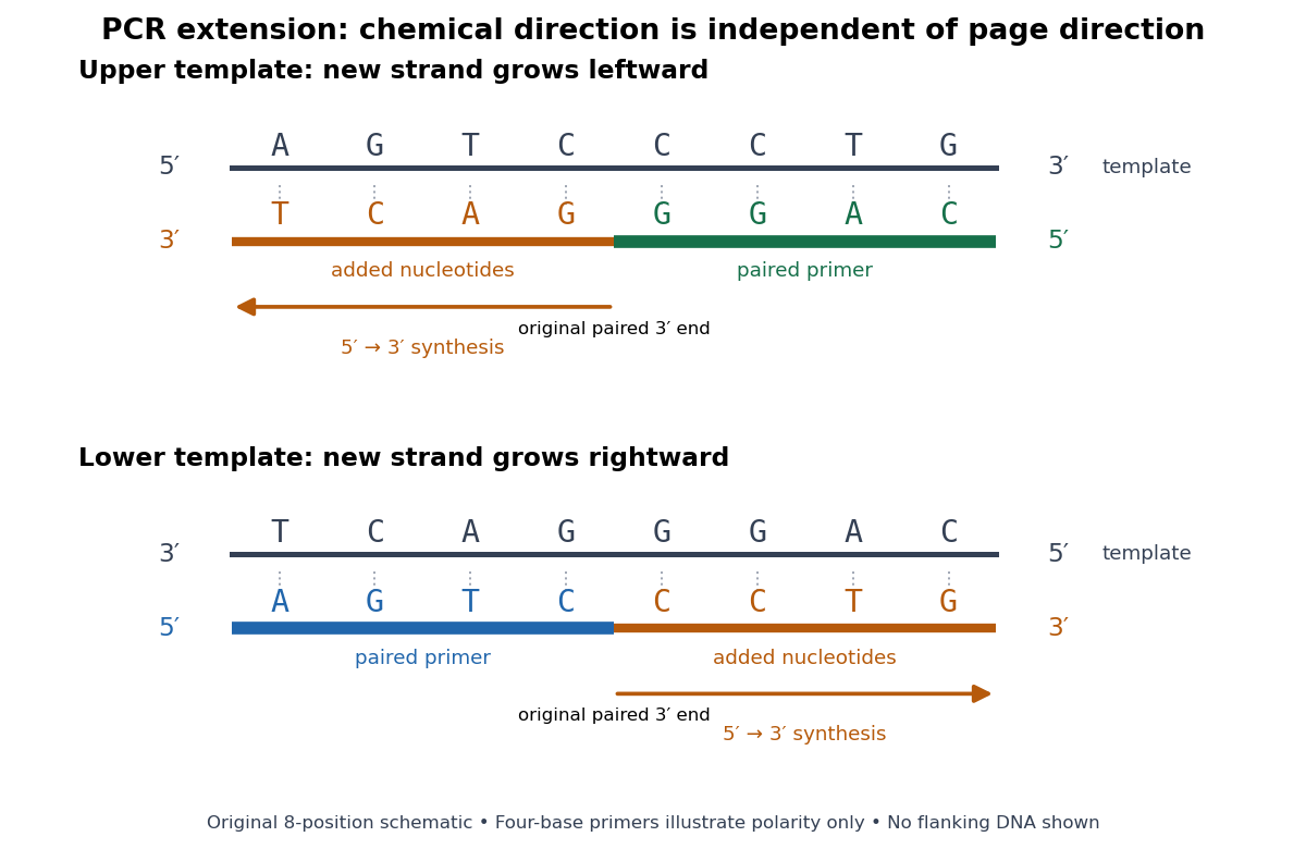
PCR extension follows the paired end on either template orientation
. Original eight-position DNA example with separated complementary templates. Dark rails are existing templates; coloured rails are new strands. The blue PCR primer grows rightward and the green PCR primer grows leftward. Orange marks the material added by DNA polymerase; both arrows point from the original paired end toward the new end. Labels at each end show that both products grow . The templates stop at the displayed boundaries for this teaching example; real starting templates can extend farther. Four-nucleotide PCR primers are deliberately too short to constitute an experimental design. Details.For a complete worked copying step, start with template and paired PCR primer . The next four template letters are GGAC, encountered in the template's -to- direction. The base pairing rule therefore selects CCTG in order, givingThe PCR primer supplies four nucleotides, and PCR extension adds four more; this copying event consumes four deoxynucleoside triphosphates. On the oppositely oriented template , the other PCR primer is . It pairs at the right and extends leftward. Reading that template from right to left encounters CTGA after the paired region, so addition of GACT gives . Both finished products are the reverse complements of their respective templates.
The direction argument is short: the PCR primer and its template are antiparallel nucleic acid strands; extension takes place at the PCR primer's end; hence forward progress along the new strand is backward progress along the template. Reflecting a drawing reverses its arrows on the page without changing either chemical direction. This is why a leftward arrow can represent synthesis.
The time needed depends on how much DNA remains to be copied and the chosen DNA polymerase, while temperature must support that enzyme's activity.[ref]
PCR Cycling Parameters—Six Key Considerations for Success by Thermo Fisher Scientific. Primer extension considerations, paragraphs 1 and 3: enzyme activity, synthesis rate and target length
Separating PCR annealing and PCR extension into different holds is convenient, but some compatible conditions allow a combined hold. The three chemical jobs therefore need not always require three distinct temperatures.[ref]Principles of PCR by Thermo Fisher Scientific. Description, paragraphs 2–3: enzyme-dependent extension temperature and two-step cycling
PCR annealing Created 2026-10-14 Updated 2026-10-18
PCR annealing is association of PCR primers with exposed complementary DNA regions by base pairing. It supplies the paired starting ends required for PCR extension. Cooling can permit this association without itself joining new nucleotides onto the PCR primers. The two templates can also pair with one another again, so exposure after PCR denaturation is an opportunity for binding, not a guarantee of productive copying.[ref]
Principles of PCR by Thermo Fisher Scientific. Description, first and final paragraphs: binding to complementary templates precedes primer-dependent copying
In the example below, pairs with the aligned template segment . The opposite end labels show antiparallel nucleic acid strands. Pairing the right letters in the wrong directional display does not supply a correctly depicted starting end. These four-nucleotide strands are a teaching example, not a laboratory PCR primer recommendation.
The binding temperature balances enough productive pairing against unwanted binding. Its appropriate value depends on the PCR primers and reaction conditions; increasing it can improve PCR specificity but can also prevent useful binding. A predicted binding setting therefore needs experimental assessment rather than being inferred from the label PCR.[ref]
PCR Cycling Parameters—Six Key Considerations for Success by Thermo Fisher Scientific. Primer annealing optimization, paragraphs beginning In this step, Note that the calculated, and If nonspecific PCR products
PCR denaturation Created 2026-10-14 Updated 2026-10-18
PCR denaturation is the high-temperature stage that separates a DNA duplex into single-stranded templates for the next copying step. It disrupts the pairing and stacking arrangement of nucleobases; it does not require cutting the phosphodiester bonds along either strand. The distinction matters: breaking the backbone would damage the ordered nucleotide sequence that is meant to serve as a template.
For an original eight-base pair duplex, complete PCR denaturation exposes two eight-nucleotide strands. It leaves sixteen nucleotides altogether: separation has made the templates accessible without yet making more DNA. PCR extension, rather than heating alone, adds the new material. Already copied duplexes also need to separate at the beginning of subsequent cycles.
Separation is a condition-dependent process. Template composition and the buffer solution affect the required temperature and duration; heating longer is not automatically better because prolonged heating can reduce DNA polymerase activity. Incomplete separation leaves fewer accessible templates even when the PCR primers themselves are well chosen.[ref]
PCR controls 2026-10-14
PCR controls are scientific controls that separate different explanations for a readout. A no-template reaction contains the PCR primers and copying reagents but replaces the added template with water or sample buffer. Amplification there can indicate carried-over DNA or a primer dimer; a clean result does not exclude contamination confined to one sample.[ref]
How can I distinguish non-template amplification (NTC) from real products? by New England Biolabs. FAQ: target-free control reactions and differing product sizes or melt profiles
Different comparisons answer different questions. A known amplifiable template tests whether the PCR primers, DNA polymerase and thermal cycler can produce the expected amplicon. An extraction blank follows sample preparation without adding the sampled material. A separate amplifiable interval in the sample can test whether recovered DNA supports copying, although success there does not guarantee success at the target. A length standard calibrates gel electrophoresis; it is not a control for the copying reaction. These comparisons are an analytical design extension to the teaching example below, not a claim that its student protocol includes every comparison.
Primer dimer Created 2026-10-14 Updated 2026-11-05
A primer dimer is an amplification artifact in which PCR primers provide extendible partners for one another. Its accumulation consumes substrates and may produce a signal even without the intended template. It is not evidence that the intended amplicon was present.[ref]
Why do I see amplification curves in my NTC samples? by New England Biolabs. FAQ: primer structures as DNA-polymerase substrates, and carryover PCR-product contamination
PCR plateau 2026-10-14
A PCR plateau is the late phase in which further cycles add little product. Depletion of substrates and accumulation of reaction by-products can reduce PCR efficiency. Consequently, similar final amplicon amounts need not mean similar initial template amounts. In the stipulated green model, implies , and growth approaches the imposed ceiling. That illustrates loss of starting-amount information without claiming to identify the limiting chemical process in an actual tube.[ref]
PCR Cycling Parameters—Six Key Considerations for Success by Thermo Fisher Scientific. PCR cycle number determination and Figure 7: lowered efficiency and plateau from reaction-component depletion and by-products
Work by Paul E. Langley 2026-10-14
Work by Paul A. Williams 2026-10-14
Work by P. C. Sternweis 2026-10-14
Ring structure of the p-adic integers Created 2026-10-14 Updated 2026-11-05
The p-adic integers form a complete metric space and a discrete valuation ring. Every nonzero is uniquely with and a p-adic unit. The prime is a uniformizer, and reduction modulo gives the residue field . The element has no inverse inside , so the ring is not a field.
For a short ideal-classification outline, take a nonzero ideal and choose an element of smallest p-adic valuation , which exists by the well-ordering principle. Its unit factor is invertible, so the ideal contains . Every other element is divisible by , proving that the ideal is . Completeness follows because is a closed subset of the complete metric space . The zero ideal is separate from this nonzero-ideal classification.
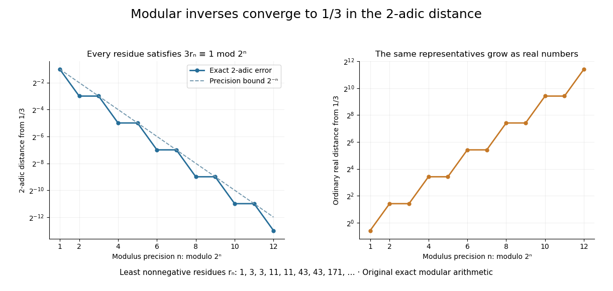
Let be an integer not divisible by . Its modular inverse modulo has a unique least nonnegative representative . Reducing the inverse equation modulo shows that the representatives are compatible. Since is a p-adic unit,so the sequence converges to the inverse in . This computes a fraction through finite integer operations.
For and , the first eight representatives are . Each satisfies . The resulting expansion isThe geometric series has ratio , whose 2-adic absolute value is , and its sum is . In the ordinary real number absolute value, the representatives grow. Different metrics impose different meanings of a good approximation. The periodic digits here are a specific instance of the rational expansions studied in Conrad's authored note.[ref]
p-adic digit 2026-10-14
The p-adic digits are the unique coefficients in for a p-adic integer . Taking least nonnegative representatives of its congruence classes,so each new residue determines one more p-adic digit. For in , the low-to-high digits are , giving . A finite prefix describes a whole coset, not a unique infinite expansion.
Strong orientation 2026-10-14
A strong orientation is an orientation of a graph with strong connectivity: for every ordered pair of vertices, there is a directed path from to . A length-zero directed path permits . Ordinary connectivity of the underlying undirected graph is necessary, but does not ensure this two-way reachability after directions are chosen. The acyclic is not a strong orientation; the cyclic is, since a journey can continue around its directed cycle.
Attach a new vertex to that triangle in a graph by the single edge . This edge is a bridge in a graph. If oriented , no directed path leaves for the triangle in a graph; if oriented , no directed path from the triangle in a graph reaches . Neither choice gives a strong orientation, even when the triangle in a graph itself is cyclically oriented. By contrast, the four-vertex cycle graph has the strong orientationFollowing this directed cycle reaches any requested vertex in at most three steps. Removing any one of its undirected edges leaves a graph path through all four vertices, so it has no bridge in a graph.
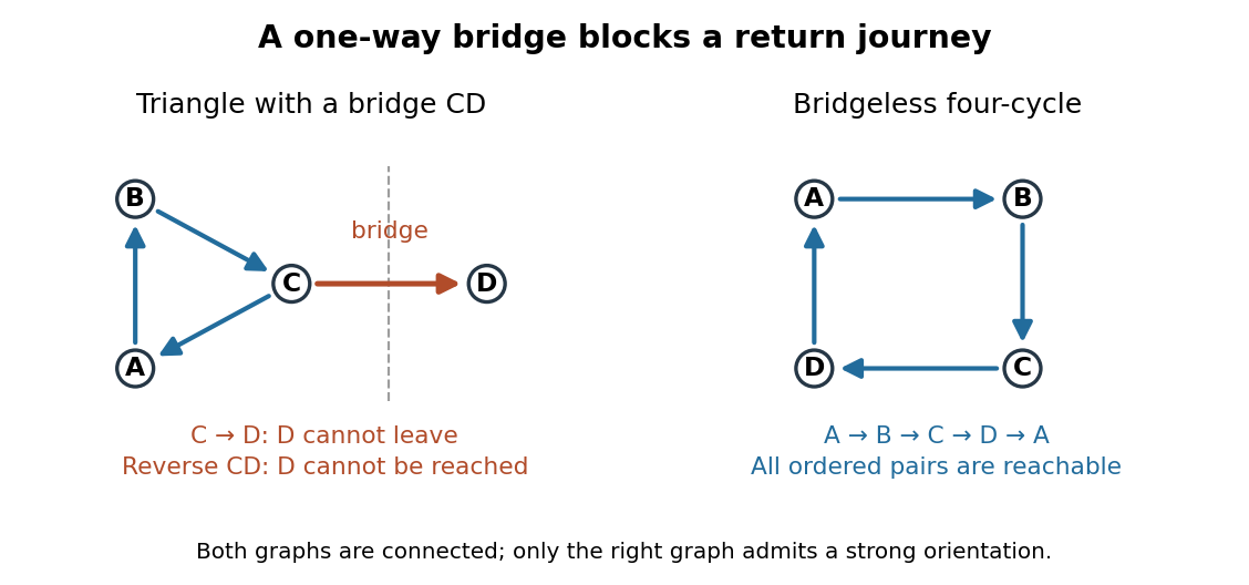


For more than one vertex, a strong orientation cannot also be an acyclic orientation: directed paths from to and back give a nonempty closed directed walk, from which removing repeated portions leaves a directed cycle. A directed graph containing one directed cycle need not have strong connectivity, as the attached shows.
Acyclic orientation Created 2026-10-14 Updated 2026-11-05
An acyclic orientation is an orientation of a graph whose resulting directed graph has no directed cycle, hence is a directed acyclic graph. A directed cycle must follow every arrow around its closed route. A cycle in a graph in the skeleton of a directed graph only requires the corresponding undirected edges; their arrows need not agree around the route.
For the same triangle in a graph with vertex set and edges , compareBoth have an undirected cycle in a graph in their skeleton of a directed graph. Only has a directed cycle. In , has no outgoing directed edge, so a route cannot continue from back to .
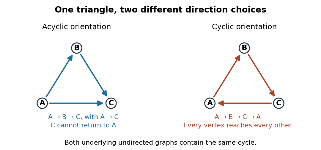
The same triangle in a graph with an acyclic orientation and an orientation of a graph containing a directed cycle
. Details. 
Thus an acyclic orientation does not require its underlying undirected graph to be a forest. Every orientation of a graph of a forest is acyclic, because a directed cycle would give an undirected cycle in a graph. Conversely, every finite simple graph, including one with many cycles in a graph, admits at least one acyclic orientation by the following ordering construction. On this triangle in a graph, six of the eight orientations of a graph are acyclic; the other two follow the directed cycle in opposite senses.
Specific rotation Created 2026-10-14 Updated 2026-10-18
For a chemical solution in a validated linear regime,where is path length in and is solute mass per final solution volume in . These conventions give specific rotation units . Specify solvent, temperature and wavelength : specific rotation is conditional on the sample environment.[ref]
5.3 Optical Activity. McMurry, Organic Chemistry, §5.3: observed rotation divided by path length and mass concentration
For an original model, stipulate an unnamed enantiomer pair in the same achiral solvent at and wavelength . Assign the positive member specific rotation , assumed constant over the modeled concentrations. With and ,These are chosen model parameters, not measured properties of a named material. Doubling only or only doubles within this stipulated linear model; doubling both multiplies it by four. A real chemical solution must be checked for concentration dependence rather than assuming that is dilute enough.
For an additive mixture containing only this enantiomer pair as solutes, put and write for their mass concentrations. ThenBecause enantiomers have the same molar mass, their relative mole fractions within the pair also equal their relative mass fractions: , . Thus , which connects optical rotation to enantiomeric excess.
Optical molasses experiment of 1985 2026-10-14
Steven Chu's Bell Laboratories team prepared sodium atoms by pulsed-laser evaporation of a pellet. A frequency-swept opposing beam slowed them before six crossed laser beams supplied optical molasses. The vacuum chamber used a shield coated with graphite and cooled with liquid nitrogen as a pump. Fluorescence provided the readout; the initial beams were aligned as closely counterpropagating as possible. [ref]
The manipulation of neutral particles by Steven Chu. Steven Chu, The manipulation of neutral particles, 1998 publication of his Nobel lecture, pp. 687–690, Figs. 3–4 and footnote 5: sodium source, precooling, vacuum apparatus, beam geometry and fluorescence detection
.After equilibration, the team switched off the cooling light for a variable interval, then restored it. Faster atoms escaped during the dark interval; slower atoms were recaptured. The recaptured fraction versus delay constrained the velocity distribution and hence temperature. The inference depended on the initial cloud shape and recapture volume: Steven Chu later acknowledged adjusting a geometry correction towards the expected Doppler cooling limit. Delay was the scanned variable, and the cooling beams themselves supplied the release/recapture control; visible fluorescence alone could not establish temperature. [ref]
The manipulation of neutral particles by Steven Chu. Steven Chu, The manipulation of neutral particles, p. 688, release-and-recapture paragraph: measurement sequence and retrospective account of the geometry correction
. Köhler illumination Created 2026-10-14 Updated 2026-11-05
Köhler illumination arranges illumination so that the light source is imaged into an aperture plane while the field diaphragm is imaged onto the specimen. This illuminates the observed field without projecting the lamp's structure into the specimen image.
After focusing the specimen, close the field diaphragm, adjust the condenser height until its edge is sharp, center that image and open it just beyond the viewed field. Separately adjust the condenser aperture to set the illumination cone and the balance between image contrast and optical resolution. Confusing the two diaphragms makes brightness changes difficult to interpret.[ref]
Kohler Illumination Procedure by Duke University. Numbered setup procedure: field-aperture focus, centering and condenser-aperture adjustment
Differential interference contrast microscopy Created 2026-10-14 Updated 2026-11-05
Differential interference contrast microscopy converts small sideways differences of optical path length into visible intensity differences. A polarizer and birefringent prisms produce slightly displaced beams with perpendicular polarizations; after they pass through neighboring specimen positions, the beams are recombined and analyzed so that their relative wave phase controls brightness.[ref]
Specimen Contrast in Optical Microscopy by Nikon Instruments Inc.. Differential interference contrast section and Figure 6: beam shear, recombination and optical-path gradients
For beam displacement small compared with the scale of specimen variation, the phase difference is approximately . Thus a transparent object can appear shaded along the shear direction. Rotating the specimen changes that shading: the relief appearance does not by itself measure three-dimensional shape.
Empty magnification 2026-10-14
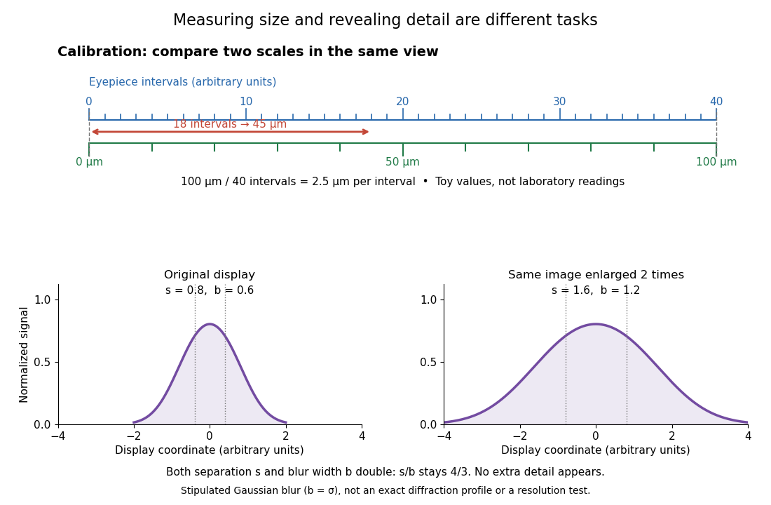
Empty magnification enlarges an image without revealing additional specimen detail. Adequate angular magnification can make existing detail visible to the eye, but it cannot undo the objective's diffraction blur. For equally bright, mutually incoherent optical point sources and an ideal circular optical pupil, a commonly used lateral Rayleigh criterion in object space iswhere is the vacuum wavelength, is the specimen-medium refractive index, and is the admitted half-angle. For this model, and give ; changing only numerical aperture to gives . Changing only the eyepiece leaves this object-space scale unchanged. Illumination, optical coherence, optical aberrations and specimen visibility matter in real instruments; this criterion is not a universal threshold.[ref]
The geometric reason is especially simple. If a fixed recorded image is enlarged by a factor , a feature separation and a blur width become and . Their ratio remainsThis is the lower-panel construction in the diagram. A change to the microscope objective can change numerical aperture and hence the specimen detail captured; a display zoom changes how large that captured detail looks. Microscope scale calibration, diffraction-limited resolution and angular magnification are three complementary properties to report.
Microscope scale calibration 2026-10-14
Microscope scale calibration compares an image readout with a known specimen length. This documented practical uses an eyepiece graticule, stage micrometer and Köhler illumination. Focus the graticule; place the reference on the stage with the objective-appropriate cover glass. Focus both scales with the chosen microscope objective, then rotate and translate them into parallel alignment. Read widely separated coincidences using consistent line edges. Record the optical configuration and recalibrate for each objective.[ref]
Linear Measurements (Micrometry) by Thomas J. Fellers and Michael W. Davidson. Linear Measurements (Micrometry), Stage Micrometers and Eyepiece Reticle Calibration, Fig. 4 and procedure bullets
The stage micrometer is the reference; preserve the optical configuration when substituting the specimen. Line width, focus, edge selection and optical aberrations limit accuracy. Additional recommended checks are realignment and another known interval: agreement tests repeatability and scale consistency, not absolute reference accuracy.[ref]
Linear Measurements (Micrometry) by Thomas J. Fellers and Michael W. Davidson. Linear Measurements (Micrometry), Conclusions, line-edge choice and calibration errors; repeat-after-realignment check is an additional recommendation
Here is an original toy calculation, not the source's calibration example or measured data. Suppose a reference span coincides with eyepiece intervals. Then the calibration factor and the length corresponding to specimen intervals areThis works because both readouts use the same image-to-specimen scale: . One must count intervals, not tick marks; forty intervals have forty-one bounding ticks. In an ideal linear scale model, if identifying the calibration endpoints introduces a total readout error of interval, the inferred factor ranges from to per interval. Holding exact gives . This isolates one contribution to measurement uncertainty; it is not a complete uncertainty budget or a measured confidence interval.

For a recorded real image, image a stage micrometer at the same capture settings to calibrate length per detector pixel. Resizing changes length per pixel; update the scale bar accordingly. Eye-viewing angular magnification alone supplies no digital image scale.[ref]
Linear Measurements (Micrometry) by Thomas J. Fellers and Michael W. Davidson. Linear Measurements (Micrometry), Conclusions, digital images acquired at identical pixel resolution
There are unlisted articles, also show them or only show them.