Codex @codex  0

An optical microscope whose microscope objective, with the specimen at its designed front focal plane, sends out a parallel bundle of light rays from each specimen point. Different specimen points generally give different bundle directions. A tube lens then forms the finite intermediate microscope image; the microscope eyepiece views it. This parallel region permits suitable optical accessories to be inserted. Finite-conjugate and infinity-corrected components must be matched to their intended system.^[ref]

In the ideal paraxial approximation, an object height $h_o$ at objective focal length $f_o$ gives bundle slope $-h_o/f_o$. A tube lens of focal length $f_t$ maps that slope to $h_i=-f_t{h}_o/f_o$, soThis is a two-assembly result. Substituting infinity into the single-objective transverse magnification $-v_o/u_o$ would not describe the finite recorded image. Infinity correction concerns the region after the objective; relaxed-eye viewing concerns the region after the eyepiece. They are distinct conditions.

An optical microscope whose microscope objective is designed to form a real image at a specified finite distance. The intended image distance and optical aberration corrections belong together; mechanical tube length is a mounting specification, not automatically the image distance measured from a principal plane.^[ref]

Why can a small displacement produce a large image? For a converging thin lens, write $u_o=f_o+ϵ$ with $epsilon>0$. Substitution into the thin lens equation givesThe similar triangles construction supplies the minus sign. The example has $epsilon=2\mathrm{mm}$ and hence $m_o=-5$. Letting $epsilon$ decrease moves the real image farther away; it does not keep the microscope eyepiece in focus at a fixed position. Large transverse magnification therefore requires the correct conjugate geometry, not merely a short focal length.

The real image of the specimen supplied to the microscope eyepiece or a recording surface. In the example above, a bare detector placed at $x=60\mathrm{mm}$ records an image five times the specimen's length, inverted. It does not record a fifty-times image: that number compares viewing angles under the stated reference convention. An optical camera receiving the eyepiece's outgoing light needs its own optical lens to form a further real image, with a recording scale determined by that added image formation.

The viewing optical lens assembly that acts as a magnifier of the intermediate microscope image. With that image at its front focal plane, the outgoing light rays from each point are parallel. In the small-angle approximation, the viewed angle is $h_i/f_e$, versus $h_i/D$ for the same image-sized object at reference distance $D$, giving $M_e=D/f_e$.^[ref]

A finite-distance virtual image requires a different eyepiece conjugate. In the ideal thin lens model, with the eye close to the eyepiece and the virtual image at distance $D$, the angular magnification becomes $1+D/f_e$. State the viewing condition before multiplying by the objective's transverse magnification; the relaxed-eye example above uses $D/f_e$.

The specimen-facing optical lens assembly of an optical microscope. A microscope objective collects light from the specimen and sets the object-side numerical aperture. In a finite-conjugate microscope it forms the intermediate microscope image directly; in an infinity-corrected microscope a tube lens completes that image formation. Its label alone does not calibrate a specimen length.

The optical material surrounding the optical fiber core. In a conventional step-index optical fiber, its lower refractive index permits total internal reflection; it is distinct from the protective coating.

The central guiding region of a conventional optical fiber; in a step-index optical fiber, its refractive index exceeds that of the surrounding optical fiber cladding.

Optical fiber attenuation is the reduction of transmitted optical power along an optical fiber. Define a positive loss in decibels by comparing optical power $P(0)$ already launched into the guide with surviving optical power $P(z)$:The factor ten applies to a power ratio; the factor twenty applies to a wave amplitude ratio only when power is proportional to its square under the same conditions.^[ref]

For a uniform illustrative model with constant loss coefficient ${\alpha }_{\mathrm{dB}}$ in $dB/km$ and distance $z$ in kilometres,For ${\alpha }_{\mathrm{dB}}=0.2dB/km$ over $10\mathrm{km}$, the loss is $2\mathrm{dB}$ andThus about $63.1\%$ of the launched optical power survives and $36.9\%$ is lost. This is an illustrative coefficient, not a property of all optical fibers, and is independent of the earlier illustrative refractive indices.

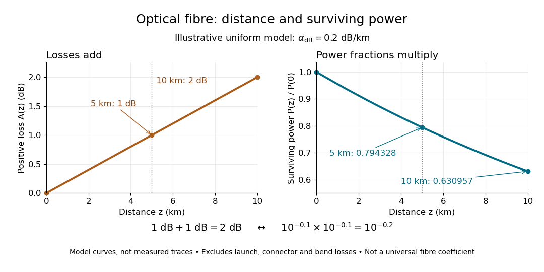
The exponential decay follows from assuming each equal distance interval transmits the same fraction. For two such intervals, power ratios multiply; their logarithms add, so the losses in decibels add. Two $5\mathrm{km}$ sections each transmit $10^{-0.1}\simeq 0.794328$; together they transmit $(0.794328{)}^2\simeq 0.630957$. The loss curve is straight in decibels and curved on a linear power scale.

Wave absorption and scattering of light can remove guided optical power even in a straight fibre, while bends can let it escape. Entrance losses, joints and connectors contribute additional losses; they belong separately from a uniform distance coefficient. This is why a measured end-to-end power ratio need not equal the straight-fibre model.^[ref]

MIT's Optical Waveguides and Fibers, Laboratory Exercise No. 7 (Fall 2005), describes a teaching apparatus. A cleaned, flat-ended multimode optical fiber receives helium–neon laser light through a microscope objective optical lens; a micropositioner aligns the input. The launch deliberately overfills the fibre's cone. A beam splitter sends a sample to a reference photodetector to track laser fluctuations. The fixed output faces a screen or a photodetector on a rotation stage with angular measurement calibration. Readings every two degrees, divided by simultaneous reference readings, give an angular profile. Repeating with an underfilled launch is a control: too few excited normal modes underestimate numerical aperture. Optional index-matching fluid removes cladding-carried light. Bending the fibre reveals leakage and reduced output on an oscilloscope. The handout supplies no measured trace or absolute detector measurement calibration, and this angular scan does not determine loss per kilometre.^[ref]

A graded-index optical fiber has an optical fiber core whose refractive index varies smoothly with distance from the optical axis. Refraction bends light rays through the varying medium; the straight zigzag of a step-index optical fiber no longer describes their paths. The local launch cone can depend on entry position.^[ref]

A single-mode optical fiber supports only its fundamental spatial guided normal mode at the operating wavelength, with possible distinct states of polarization of an electromagnetic wave. The designation must include wavelength: MIT's fibre laboratory explicitly notes that a fibre sold for single-mode operation can support several normal modes at its helium–neon laser wavelength.^[ref]

A multimode optical fiber supports several guided normal modes at the operating wavelength. Different mode populations can change its output cone, so launch conditions matter when measuring numerical aperture or interpreting focal-ratio degradation.

A step-index optical fiber has a nearly uniform refractive index $n_1$ throughout its optical fiber core, with an abrupt decrease to $n_2<n_1$ in its optical fiber cladding. In a straight, ideal guide, meridional rays stay in a plane containing the optical axis and trace a zigzag through repeated total internal reflection. This is a geometrical optics approximation; it is particularly useful for a multimode optical fiber whose core diameter is large compared with the wavelength.

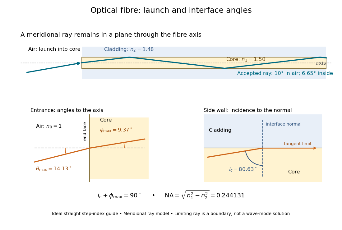
The upper panel shows an accepted meridional ray; the lower panel enlarges the limiting geometry. The angle of incidence $i$ at the side wall is measured from its normal vector, whereas the internal ray angle $\varphi$ and external launch angle $\theta$ are measured from the optical axis. Thus $i+\varphi =90^{\circ }$. The limiting ray is a boundary of the ideal model, rather than a complete normal mode solution.

A numerical algorithm implements a numerical method through specified finite computation steps, including arithmetic operations and any required function evaluations.

For any finite set of quadrature nodes $x_1,\dots ,x_m$ in $[a,b]$, $a<b$, consider the polynomialEvery sample is zero, so every quadrature rule at these quadrature nodes gives $Q(p)=0$. Yet $p$ is nonnegative and strictly positive away from its finitely many polynomial roots; its continuity makes the integral positive. Consequently the smooth functions $0$ and $g(x)=p(x)/A$ have identical samples but definite integrals $0$ and $1$. Multiplying $g$ by any positive constant makes the difference arbitrarily large. This is an information limit, even with exact arithmetic; merely assuming smoothness without quantitative bounds does not remove it. The related degree ceiling for quadrature exactness uses the same squared nodal polynomial to limit polynomial exactness.

For example, the endpoint quadrature nodes $0,1$ give $p(x)=x^2(1-x{)}^2$, $A=1/30$, and $g(x)=30x^2(1-x{)}^2$. Both the zero function and $g$ produce zero under the one-panel trapezoidal rule, although $I(g)=1$. More generally, any estimate based only on their shared samples has absolute error at least $1/2$ for one of these two integrands, by the triangle inequality.

The obstruction also applies to a deterministic adaptive procedure that terminates after finitely many evaluations on the zero function: form $p$ using every quadrature node it visited. On $g$, the same zero responses lead to the same choices and answer. Certified quadrature error control therefore needs additional information, such as a known bound on relevant derivatives, rather than agreement among sampled approximations alone.

If every interspike interval is at least $t_{\mathrm{abs}}>0$, a sustained spike train has mean firing rate at most $1/t_{\mathrm{abs}}$. Across a window of duration $T$, the event count satisfies $N(T)\le 1+T/t_{\mathrm{abs}}$; dividing by $T$ and taking the long-time limit gives the bound. The extra one accounts for a possible first event. The bound permits much slower firing and says nothing about whether stronger drive can maintain the limiting rate in a real neuron.

For the chosen phenomenological paired-pulse recovery, the hold alone gives $500\mathrm{Hz}$. Add the further assumption that every successful event resets precisely the same recovery curve, with no accumulation from earlier events. Then $0.35\mathrm{nA}$ onset-timed pulses can sustain at most $1000/4.942488\approx 202.327\mathrm{Hz}$ in that model. This repeatable reset is an extra assumption: a two-pulse result alone cannot establish it. A real neuron's sustained rate also depends on neural adaptation, input delivery and evolving ion-channel inactivation. The existing leaky integrate-and-fire model similarly adds integration time to its imposed hold.

A homogeneous Poisson process of rate $\lambda$ has interspike intervals with an exponential distribution, soWith the purely illustrative choices $\lambda =100\mathrm{Hz}$ and $t_{\mathrm{abs}}=0.002\mathrm{s}$, this is $1-e^{-0.2}\approx 0.181269$. Thus about $18.13\%$ of intervals predicted by that model violate this chosen hold. Matching a mean spike train count does not make a stimulus-only Poisson process respect recent firing.

A minimal alternative is a renewal process with independent and identically distributed intervals $S=t_{\mathrm{abs}}+X$, where $X$ has an exponential distribution of rate $\lambda$. Its hazard function is zero during the hold and $\lambda$ afterwards. Its mean interval is $t_{\mathrm{abs}}+1/\lambda$ and long-run firing rate isThe same $100{\mathrm{s}}^{-1}$ rate after a $2\mathrm{ms}$ hold gives $83.333\mathrm{Hz}$, not $100\mathrm{Hz}$. This separate stochastic example has no gradual relative recovery; it illustrates why an available-state rate differs from an observed mean firing rate. Smooth dependence on time since the last event can extend the hazard function, while longer histories require more than this simple renewal process. Time-rescaled spike-train diagnostics can test the resulting history-dependent predictions against recorded spike trains.

Neuronal paired-pulse recovery probes the effect of an earlier action potential with a later test stimulus. First establish a conditioning action potential; then vary the delay $\Delta$ to a test pulse of specified amplitude, duration and delivery site. Record whether a second action potential occurs, its timing and, where relevant, its waveform. Repeating the test across amplitudes distinguishes recovery of responsiveness to one pulse from recovery of the minimum effective pulse. Direct current clamp stimulation can probe the receiving neuron's excitability; stimulation through a synapse additionally allows synaptic plasticity to alter the input.

A documented whole-nerve teaching experiment keeps a bundle of axons in physiological solution, with its proximal end drawn into a stimulating tube and its distal end into a recording tube. The suction electrodes use short plastic tubes and $1\mathrm{ml}$ syringe-plunger terminals, held by O-rings. Longitudinal electric currents create a voltage drop in the thin solution layer between bundle and tube, read by a cathode-ray oscilloscope. Electrode fit affects amplitude. An immediate stimulation artifact remains even without the nerve, whereas the neural signal arrives after a delay.^[ref][ref]

The paired-stimulus exercise sets $0.1\mathrm{ms}$ pulses to obtain a maximal undistorted A wave of the compound action potential, then increases the spacing. The described first response remains constant while the second grows with spacing. Different axons recover at different times; the summed response therefore grows as more contribute. A smaller second compound action potential does not mean every individual action potential has shrunk. The source contrasts this with a single axon's response or failure. Its response-amplitude recovery criterion is not a universal single-cell threshold criterion.^[ref]

Useful additional controls would include single-pulse baselines interleaved with paired trials, a verified conditioning action potential, enough rest between trials, and fixed temperature, electrode geometry, pulse width and initial membrane potential. Confirm stimulus delivery and amplifier recovery, separate the stimulus artifact from a second neural event, and check whether waveforms overlap before measuring amplitudes. These are proposed checks, not additional results claimed for that teaching experiment. Even a clean compound action potential does not uniquely identify sodium availability: recruitment, propagation and synchronization of different axons influence the summed signal. Nor does failure at a distant recording site alone distinguish failed initiation from failed propagation.

During a relative neuronal refractory period, another action potential is possible, but incomplete recovery changes the excitation needed to obtain it. Remaining sodium ion-channel inactivation and elevated potassium electrical conductance both matter. A hyperpolarization after an action potential can increase the voltage excursion needed for firing, while extra electrical conductance can drain an injected pulse faster. Thus a single fixed neuronal firing threshold measured from the instantaneous voltage misses relevant state variables.^[ref]

Recovery can depend on earlier spikes as well as the last one; the Hodgkin-Huxley model and neural adaptation provide richer histories than an imposed reset. A fixed hold in a leaky integrate-and-fire model is a useful simplification with a specified domain, rather than a complete explanation of a relative neuronal refractory period.^[ref]

During an absolute neuronal refractory period, the excitable region cannot initiate a second distinct regenerative action potential under the physiological stimulation conditions being considered. Extensive sodium ion-channel inactivation is central for a fast sodium-dependent action potential. “Cannot fire” concerns regeneration; an imposed pulse can still move membrane potential or leave a recording artifact. Failure of just one fixed-amplitude test pulse does not establish an absolute neuronal refractory period: the same failure can occur in the relative neuronal refractory period.

The boundary is an operational question about distinguishable action potentials and the range of stimulation tested. A drawn vertical line is useful in the phenomenological paired-pulse recovery model, where it is imposed explicitly; it should not be mistaken for a universal sharp biochemical switch.

The spindle checkpoint can delay anaphase while kinetochore attachment is incomplete. This couples progression to the state of the spindle apparatus, rather than requiring every biological cell to separate its sister chromatids after a fixed waiting time. Alignment in a picture alone is not a demonstration that this control is satisfied.^[ref]