
Triangulation of a convex polygon Created 2026-10-14 Updated 2026-10-20
A triangulation of a convex polygon divides a convex polygon into triangles using diagonals between its existing vertices of a polytope, with no diagonal crossings in the interior. For vertices it uses diagonals and produces triangles. Fixing one boundary edge, its adjacent triangle separates two smaller polygon regions; summing over the possible third vertices of a polytope gives the Catalan recurrence. Thus the number of triangulations of a convex polygon is , with the Catalan number. A quadrilateral has two choices and a pentagon has five.
Control-point influence on a curve 2026-10-14
For a parametric curve represented by fixed scalar functions and control points in Euclidean space, writeThe influence function of this handle is : the resulting displacement vector is , and its norm is . These are exact finite changes, not only a first-order estimate. Where is negative the displacement points opposite to . Where , the curve is unchanged at that parameter.
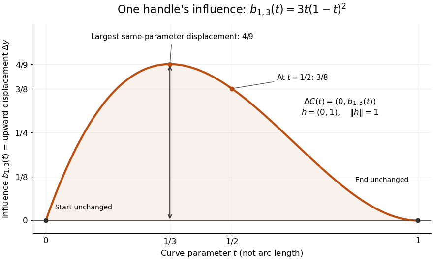
The influence coefficient 3t(1-t)^2 equals the vertical displacement for a unit upward move of P1, reaches 4/9 at t=1/3, and vanishes at both endpoints
. Details. 
For the cubic Bézier curve above, the Bernstein basis influence function is . Its derivative isIt increases up to and decreases thereafter on . Consequently the largest displacement at corresponding parameters isFor it is . This is a comparison at the same parameter. A geometric closest-distance comparison, as in a closest-point search on a subdivision curve, instead minimizes over another parameter:The closest parameter can differ from , so is not automatically a maximum closest-distance separation of the two curves. Neither parameter is assumed to be arc length.
The support of a function is the closure of the parameter values where . It bounds where a nonzero handle move can act, but may include boundary points where the actual displacement is zero. Here the support of a function is all of relative to the parameter domain, while the endpoints are unaffected. In contrast, a B-spline of order has support within in its spline knot sequence, so its handle affects only that parameter range; the support and Gram bandwidth of B-splines describes the same locality in another application. Changing the spline knots or the basis along with the handle requires a different comparison.
When the basis functions form a partition of unity, , each evaluation is an affine combination of the control points. Applying an affine map to all handles givesThis is affine equivariance of a geometric basis, also called affine covariance: affine maps preserve affine combinations. In particular, translating every handle by translates the whole curve by , whereas moving just one handle produces . The Bernstein basis has this partition of unity property.[ref]
Curves and Surfaces in Geometric Modeling: Theory and Algorithms by Jean Gallier. §4.3, pp. 132–133: Bernstein weights sum to one
Nonnegative weights further make evaluations convex combinations, giving the convex hull bound illustrated by the control polygon; nonnegativity is not needed for affine covariance.For a proof outline of the influence formula, subtract the two basis representations: every unchanged coefficient cancels, leaving . The same subtraction with several moved handles gives . No claim about interpolation, closest-point search on a subdivision curve or endpoint motion follows until the actual basis values are examined.
Work by Colin W. Taylor 2026-10-14
Static friction on an inclined plane 2026-10-14
An inclined plane tilted slowly from horizontal turns a coefficient of static friction into a critical angle. Assume a nonrotating block on a stationary, rigid, dry surface, with gravitational weight and the contact forces as its only forces. Take to be the angle between the uphill surface direction and horizontal. Let be a unit vector pointing uphill and a perpendicular unit vector pointing outward from the surface. Resolving the gravitational weight givesThe angle between the downward vertical and the inward normal is also . Thus the inward component uses cosine and the downhill component uses sine. These are components of one force, not two additional forces.
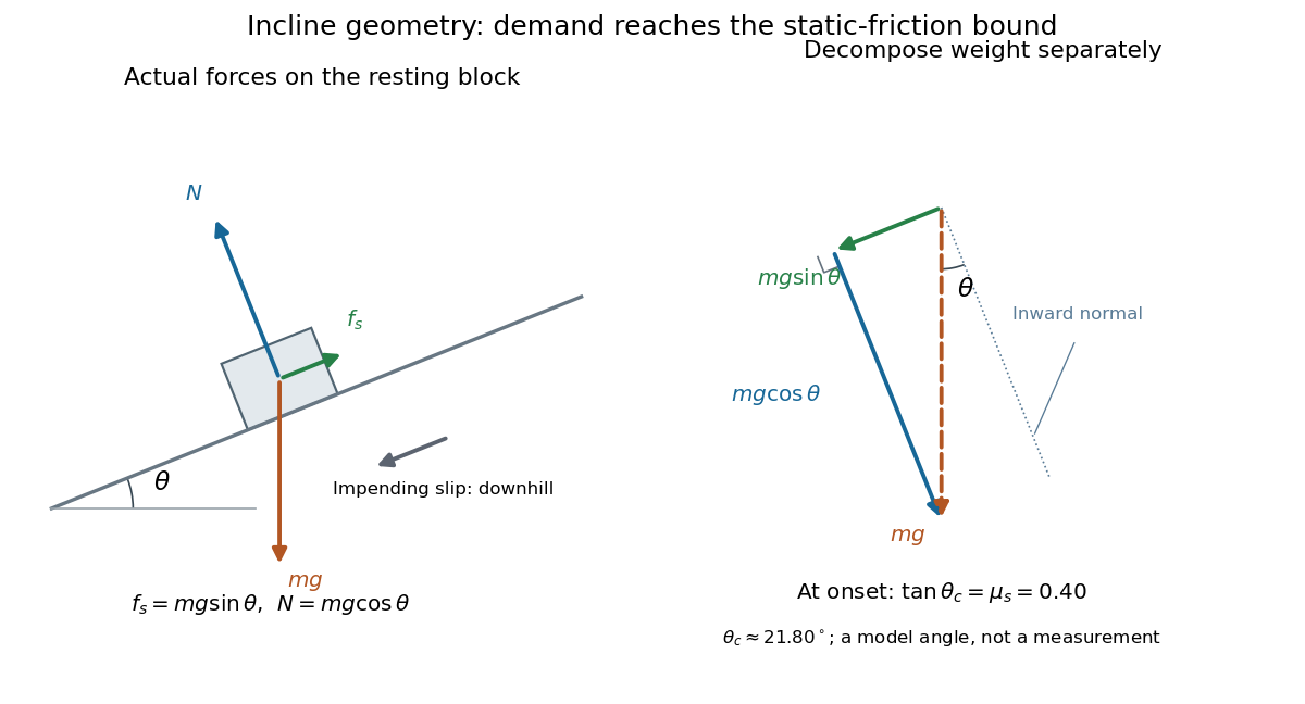

Before downhill contact slip, zero acceleration and Newton's second law requireThe required static friction points uphill. Substituting into the bound and dividing by the positive givesThe tangent function increases on this range of angles, so the last admissible resting angle isThe inverse tangent takes a dimensionless quantity to an angle. At equality the ideal model still permits a limiting resting state; increasing further excludes it. At a smaller angle, is the demand ratio, not the coefficient of static friction.[ref]
For the stipulated , and , the critical angle is approximately . At , and , comfortably below the bound . At , maintaining rest would require , but the bound is only : rest is impossible. At , and . Notice that the limiting tangential force here is smaller than the horizontal limit because tilting reduces the normal force.
Cancellation of mass makes this relation useful: the ideal critical angle tests a contact coefficient without needing a calibrated force gauge. Doubling the block's mass doubles both demanded static friction and its bound, leaving unchanged if is unchanged. This is a testable model prediction. It need not survive a change in surface condition, a direction-dependent coefficient, appreciable deformation, or vibration.
The derivation also assumes continued contact and that sliding occurs before tipping or rolling without slipping. The resultant contact force must act within the supporting footprint so that the block can satisfy torque balance; a tall block may tip first. No extra tension, imposed tangential pull, or lift is included. In a slowly raised apparatus, quasistatic process means that motion of the board contributes negligible inertial forces while locating the threshold. Once downhill contact slip begins, a constant-velocity sliding angle would concern kinetic friction, not the onset of static friction.
A clique records pairwise relationships. If vertices represent sets and an edge means a nonempty intersection, a clique does not by itself guarantee an element common to every set. TakeThen , and , so their intersection graph is . But . The graph faithfully records all three pairwise intersections; the stronger claim of a single shared element requires additional hypotheses.
Maximum clique Created 2026-10-14 Updated 2026-10-31
A maximum clique is a clique with the greatest possible number of vertices in the graph. Its size is the clique number. Every maximum clique is a maximal clique, since adding a vertex would produce a larger clique. A graph can have several maximum cliques; the word maximum specifies their common size, rather than uniqueness.
History of Catalan enumeration 2026-10-14
Leonhard Euler's 1751 correspondence already studied triangulations of a convex polygon and gave a closed formula for their counts. Johann Andreas von Segner supplied a combinatorial recurrence relation in a paper written in 1758. Eugène Charles Catalan's nineteenth-century work connected the formula to bracketed products. This history, documented in Igor Pak's account, shows how the same counting structure reappeared through different objects; the modern name alone does not establish discovery priority.[ref]
History of Catalan numbers by Igor Pak. §§2–3 and §5, printed pp. 2–4: Euler correspondence, Segner recurrence and Catalan's bracketed products
Binary parenthesization 2026-10-14
A binary parenthesization specifies the order of binary operations on a fixed ordered list of operands, combining exactly two existing expressions at each step. It has a full binary tree as its expression structure: operands are leaves and operations are internal vertices. For four operands , the five possibilities are , , , , and .
A binary parenthesization of operands contains binary operations. At the last operation, its left expression can contain operations and its right expression . The Catalan recurrence therefore gives possible evaluation structures. The order of operands stays fixed; this is not a count of their permutations. Even for an associative operation whose result is unchanged, different structures can have different evaluation costs, as in the matrix-chain multiplication problem.[ref]
Bijective Proof Problems by Richard P. Stanley. §5, Problem 154, printed p. 38: binary parenthesizations of n+1 letters
Catalan recurrence Created 2026-10-14 Updated 2026-10-20
The first-return decomposition of a Dyck path and the rule of product giveFor a given , choose the inside path in ways and its suffix in ways. Different first-return locations give disjoint groups, so the rule of sum adds their counts. For , the terms are . Iterating the recurrence relation computes the counts without enumerating every full path.
Ovary (botany) 2026-10-14
Style (botany) 2026-10-14
In the l2 sequence space, let have value one in coordinate and zero elsewhere. This orthonormal sequence is bounded: . For distinct indices , its terms obey . No subsequence can therefore be a Cauchy sequence, so none converges in the norm. Thus even a complete metric space can have a bounded sequence with no convergent subsequence. Finite dimension is essential to the usual Euclidean space extension, and in a general metric space the relevant replacement is compactness or total boundedness together with completeness.
The rational numbers lie in and obey . They form a convergent sequence in the real numbers, with limit of a sequence . Every subsequence has that same real limit. Because is an irrational number, no subsequence converges to a point in the rational numbers with their usual metric. Boundedness alone therefore does not give the corresponding theorem in every metric space; completeness of the real numbers is doing real work here. The floor function simply truncates the decimal expansion in this example.
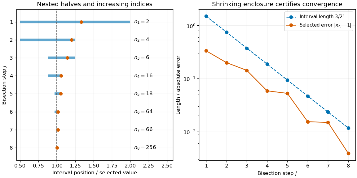
Begin with a closed interval containing the entire bounded sequence. Split the interval at its midpoint. At least one of the two closed halves contains infinitely many indexed terms; choose such a half and repeat. This gives nested intervals with lengths . The nested interval theorem, using completeness of the real numbers, supplies their unique common point .
Choose with . Infinitely many indexed terms in guarantee that the next index can be chosen. Both and belong to , soThis is a short existence proof, not necessarily a finite algorithm for an arbitrary input sequence: deciding which half contains infinitely many future terms may require mathematical knowledge about that sequence.

Choosing a different block pivot 2026-10-14
An invertible matrix need not have an invertible chosen diagonal block. For example,has singular matrices as both one-by-one diagonal blocks. Neither diagonal-block formula applies in that partition. Interchanging the two rows produces the identity matrix and a usable pivot element. This is why a failed block pivot is not proof that the full matrix is a singular matrix; Pivoted LU decomposition changes the order before eliminating.
Conversely, invertible diagonal blocks do not suffice: has but Schur complement , so it is a singular matrix. Both hypotheses in the block matrix inverse formula have work to do.
Block elimination 2026-10-14
Write a linear system as and , with an invertible matrix. Solving the first equation for and substituting in the second givesThus the Schur complement is the coefficient matrix remaining after the variables have been eliminated. When it is an invertible matrix, solve the reduced linear system for and recover . In computation, expressions such as mean solving with each column of , using the same LU decomposition or Cholesky decomposition when applicable.
For the example under block matrix inverse and right-hand side , take and . Since , the reduced equation is . Back substitution givesThe original equations return , and , respectively. The reduction retained the influence of on through the correction .
A short proof outline also explains whether is an invertible matrix: the exact matrix factorizationhas invertible matrices on the outside. Therefore is an invertible matrix precisely when the central block diagonal matrix is one. Reversing the factors gives the block matrix inverse, while taking determinants gives the Schur complement determinant identity.
Berge's theorem 2026-10-14
For a finite simple graph and a matching in a graph , is a maximum cardinality matching if and only if has no augmenting path in a matching relative to . The graph need not be a bipartite graph, and the assertion concerns cardinality, not edge benefits.[ref]
Two theorems in graph theory by Claude Berge. Claude Berge, Two theorems in graph theory, printed p. 842: finite unoriented graph and Problem 3; printed p. 843, Theorem 1: maximum matching and absence of an alternating chain between neutral points
The criterion turns a global comparison with every competing matching in a graph into a search for one repair. Starting from any matching in a graph, repeatedly find and toggle an augmenting path in a matching. Each step adds one selected edge, so finiteness gives termination after at most steps; absence of any further augmenting path in a matching certifies maximum cardinality. This is an optimality criterion, not by itself a bound on the work needed to find each graph path.
For a short proof outline, an augmenting path in a matching immediately contradicts maximum cardinality. Conversely, if another matching in a graph has , consider the subgraph whose set of edges is . Its vertices have degree of a vertex at most two; its nontrivial connected components are graph paths and even cycles in a graph, alternating between the two matchings in a graph. A cycle in a graph contributes equal numbers from each. Hence some graph path contributes one more edge from than from and starts and ends with edges from . Its endpoints are unmatched vertices in a matching relative to , yielding the required augmenting path in a matching.
Work by Arthur Pentland Dempster Created 2026-10-14 Updated 2026-10-25
An actual teaching setup is described in Laboratory Exercise No. 4: Diffraction, MIT 6.237, Fall 2024, for MIT's 6.237 Modern Optics Project Laboratory, Fall 2024. Preparation includes predicting the aperture-size dependence and the distinction between Fraunhofer diffraction and Fresnel diffraction. A helium–neon laser supplies light; the far-field setup uses a planar incident wavefront, a diffracting object and a distant screen, with beam expansion when needed. Figure 1 also marks an optional CCD camera. Exercise 4.7 asks students to sketch the circular-aperture pattern, measure the Airy disk diameter between correctly identified boundaries, and infer the aperture size. No measured values are supplied. As a regime comparison, exercise 4.9 varies the circular opening's position near a microscope objective optical lens, observes near-field patterns and compares them with the far-field case. This tests whether a change in propagation geometry changes the pattern. The coherent illumination measures one aperture's response, rather than the discrimination of two mutually incoherent optical point sources.[ref]
For a quantitative interpretation, let be the aperture-to-screen distance and the first-zero diameter on the screen. In the paraxial approximation, the independent calculation isFor an explicitly hypothetical measurement, and at would imply . The scale is smaller than , but only by a factor of about ; this alone gives limited confidence in a high-precision Fraunhofer diffraction approximation. It is not a reported MIT measurement.
Additional recommended controls are to keep wavelength fixed, record , centre and uniformly illuminate the aperture, and repeat with another . Compare , which should vary inversely with . A camera readout should include blocked-beam background and avoid saturation. A scaled repetition at larger tests residual Fresnel diffraction; nonuniform illumination, optical aberrations, detector sampling and uncertainty in locating a dark ring limit the inferred . The screen pattern's apparent bright edge depends on display brightness and is not a substitute for the first-zero boundary.
Airy disk normalization and encircled energy 2026-10-14
Peak normalization does not make the integral of a point spread function equal to one. In the paraxial approximation to the focal plane, define and . The unit-integral point spread function normalization isHere has units of inverse area; multiplying by the detected radiant flux gives image-plane irradiance. Its encircled energy, meaning the fraction inside radius , isThis is an integral over area, so its radial weight is . An unweighted integral of a line through the centre is a different quantity.
A short proof uses the Bessel function of the first kind identities and . They giveBoth expressions for vanish at zero. Since these Bessel functions of the first kind tend to zero as , , establishing the normalization. At the first dark ring,A circular detector region ending at the first zero therefore misses about of the ideal radiant flux, even though the surrounding rings have low peak light intensity. This matters when converting measured counts into total source brightness or choosing an image aperture for a photodetector.
There are unlisted articles, also show them or only show them.