
Mitotic daughter chromosome accounting 2026-10-14
Count the same hypothetical diploid animal biological cell in three ways: chromosomes, double-stranded DNA molecules, and nuclear DNA amount. Assume one continuous double-stranded DNA molecule per unreplicated chromosome or replicated chromatid, complete S phase, and no losses or mutations. Exclude mitochondrion DNA. Here is the size of one haploid set, and is its unreplicated nuclear DNA amount, as defined in cell-cycle DNA content. A double-stranded DNA molecule counts as one, despite containing two strands.
| Stage and compartment | Chromosomes | Double-stranded DNA molecules | Nuclear DNA amount |
|---|---|---|---|
| One G1 phase parent | 4 unreplicated | 4 | |
| One prophase or metaphase biological cell | 4 replicated | 8 in 4 pairs of sister chromatids | |
| Whole undivided anaphase biological cell | 8 separated daughter chromosomes | 8 | total |
| One anaphase pole's allocation | 4 daughter chromosomes | 4 | allocated |
| Each daughter after mitosis and cytokinesis | 4 unreplicated | 4 | each |
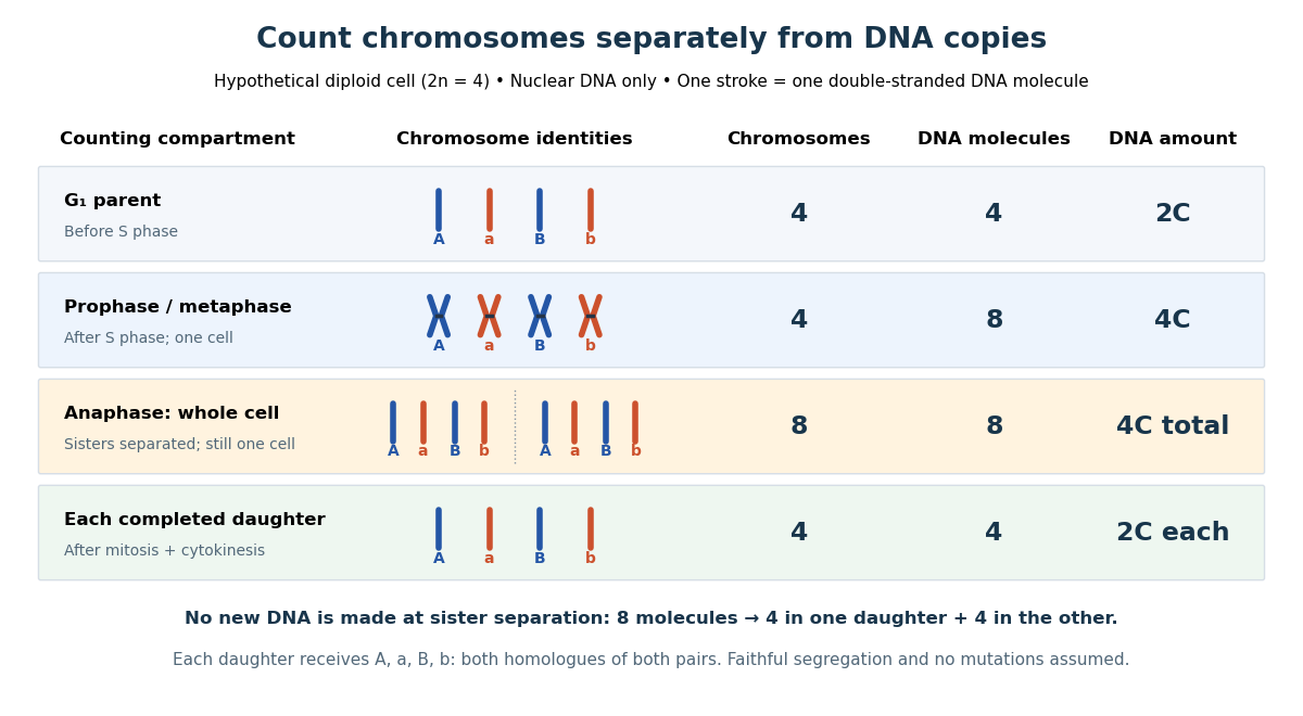

The allocation can be checked copy by copy. DNA replication turns into , into , and similarly for . One daughter receives and the other . Each therefore inherits the same four chromosome identities and the same gene and allele content as the unreplicated parent, under the stated assumptions. Across both daughters there are DNA molecules and : partition conserves the material present after S phase.
The transient whole-cell count of eight does not mean that each daughter's ploidy has doubled. Each completed daughter is diploid, containing both homologues of each homologous chromosome pair. This differs from separating homologous chromosomes during meiosis I. Faithful mitosis preserves a nuclear genome through growth and renewal; equal inherited genes need not imply equal gene expression or equal cell fate. Mutations or chromosome segregation errors can break the ideal inheritance pattern.
Telophase Created 2026-10-14 Updated 2026-10-18
In open mitosis, telophase includes reassembly of nuclear envelopes around the separated chromosome groups and relaxation of their condensation.[ref]
Metaphase 2026-10-14
In metaphase, replicated chromosomes align near the spindle apparatus equator, with their two sister chromatids connected through kinetochores toward opposite poles.
Prometaphase 2026-10-14
In open mitosis, nuclear envelope breakdown permits spindle apparatus microtubules to reach kinetochores at centromere regions.
Prophase Created 2026-10-14 Updated 2026-11-05
Condensation helps organize replicated chromosomes for later separation, while spindle microtubules begin to establish the division apparatus. Prophase precedes the stage at which all chromosomes are aligned; condensation alone is therefore not evidence of correct spindle attachment. [ref]
Work by Michael D. Tharp 2026-10-14
Same eigenvalues do not imply similarity 2026-10-14
Consider the diagonal matrix and a Jordan blockBoth have characteristic polynomial , trace , determinant , and eigenvalue with algebraic multiplicity two. But is the whole plane, whereas vanishes only when . Their eigenspaces have different dimensions, so eigenvectors under similarity rules out matrix similarity. There is an even shorter proof: for every invertible matrix .
The missing information is how the linear operator acts beyond its eigenvectors. Here , while but . Their minimal polynomials are respectively and . Over a field where the characteristic polynomial splits, the full sizes of the Jordan blocks, encoded by the Jordan normal form, determine the matrix similarity class.
Eigenvectors under similarity 2026-10-14
Under , an eigenvector in old coordinates becomes in new coordinates. Indeed,Since is an invertible matrix, the new coordinate vector is nonzero. The inverse conversion proves that the two eigenspaces have the same dimension, hence the same geometric multiplicity.
For , the eigenvector has eigenvalue . In the oblique basis of the opening example, its coordinate vector isThe tuple changes from to , but reconstruction gives : the physical vertical direction is unchanged. Calling the eigenvectors unchanged is accurate only for the underlying vectors, not for their coordinate vectors.
Matrix similarity invariants Created 2026-10-14 Updated 2026-10-25
Matrix similarity invariants are quantities unchanged by replacing with . Important examples are the characteristic polynomial, trace, determinant, matrix rank, and eigenvalues with their algebraic multiplicities. The characteristic polynomial convention here is , where is the identity matrix.[ref]
Linear Algebra Done Right by Sheldon Axler (4th edition). §9C, Definition 9.63, printed p. 363; Theorem 9.65, printed p. 364: characteristic polynomial, trace, and determinant
The short determinant proof works over any field: because , multiplicativity of the determinant givesThus its roots, the eigenvalues, retain their algebraic multiplicities in any field extension where the polynomial splits. Also . The cyclic property of the trace gives ; equivalently, the trace is determined by the coefficient of in the characteristic polynomial for an -by- matrix.[ref]
Linear Algebra Done Right by Sheldon Axler (4th edition). §8D, Theorems 8.49–8.50, printed pp. 326–327: cyclic trace identity and basis independence
For the two matrices in the opening example,Their entries differ, yet these quantities agree. Agreement is a useful necessary test for matrix similarity; it is not sufficient in general, as same eigenvalues do not imply similarity illustrates.
The relation also preserves repeated application. Adjacent factors cancel to giveFor the opening example, matrix powers therefore have the explicit formAt , this is . Acting on gives , which reconstructs as . More generally for every polynomial , so the minimal polynomial is also unchanged. Multiplication by invertible matrices preserves matrix rank, giving another invariant without finding eigenvalues.
Maximum-weight matching 2026-10-14
Assign each edge a real benefit . A maximum-weight matching maximizes over all matchings in a graph ; the empty matching in a graph is allowed. Setting every recovers a maximum cardinality matching, but otherwise the objectives can disagree.
On the same path graph , give the middle edge benefit and each outer edge benefit . The matching in a graph has total benefit , while the two-edge matching in a graph has total benefit . Thus the smaller choice is the unique maximum-weight matching. If instead the requirement is to find a maximum cardinality matching and then maximize benefit among those, the outer edges must be chosen. Requiring a perfect matching before optimizing cost is another distinct problem, covered by minimum-weight perfect matching. With negative benefits a maximum-weight matching can even be empty, so it need not be a maximal matching.
Maximum cardinality matching 2026-10-14
A maximum cardinality matching is a matching in a graph with as many edges as any matching in a graph of the same graph. It has cardinality , the matching number, and need not be unique or be a perfect matching. For example, any single edge of a triangle in a graph is a maximum cardinality matching, but leaves one vertex unmatched. Berge's theorem characterizes these optima by the absence of an augmenting path in a matching.
Alternating path in a matching 2026-10-14
An alternating path in a matching is a graph path whose successive edges alternate between membership in and membership outside . Here graph paths have no repeated vertices. Alternation alone does not make a graph path an augmenting path in a matching: its endpoints must both be unmatched vertices in a matching. For example, relative to in the six-vertex path graph, alternates but has matched endpoints; toggling just those three edges loses one selected edge.
Matching saturation 2026-10-14
A matching in a graph saturates a specified vertex set when every vertex of is incident to one selected edge. Exactly one selected edge meets each such vertex, since matching edges have disjoint endpoints. Vertices outside may remain unmatched. A perfect matching saturates the entire vertex set; Hall's marriage theorem tests matching saturation of a specified side in a finite bipartite graph.
Unmatched vertex in a matching Created 2026-10-14 Updated 2026-10-25
A vertex is an unmatched vertex in a matching if no edge of is incident to it. It is also called free or exposed, always relative to the specified matching in a graph: changing can change which vertices are free. The endpoints of an augmenting path in a matching must be distinct unmatched vertices in a matching before the change.
Work by Martha Hotz Vitaterna 2026-10-14
Work by M. J. Solomon 2026-10-14
Work by M. D. Smigel 2026-10-14
Work by Luigi Iacomini 2026-10-14
Mei-Sywe Hwang Created 2026-10-14 Updated 2026-11-05
Mei-Sywe Hwang is identified as a statistician at the Center for Measurement Standards in Hsinchu, Taiwan, in a 1993 conference paper reprinted by NIST in 1994. The coauthored report examines electronic balances for gravimetric measurements, including solid and liquid density, pycnometer calibration and mass. Its examples connect a physical instrument's readings with corrections and uncertainty in an inferred quantity.[ref]
The Electronic Balance and Some Gravimetric Applications (The Density of Solids and Liquids, Pycnometry and Mass) by Randall M. Schoonover and others. Printed p. 299, author role/affiliation, keywords and abstract; report cover, February 1994
The byline establishes her participation and historical affiliation; it does not identify an individual contribution to each experiment or establish later positions. The technical setting illustrates why measurement error and calibration are substantive parts of applied statistical work.
Shalabh Created 2026-10-14 Updated 2026-11-05
Shalabh works on statistical models whose assumptions reflect complications in observed data. His IIT Kanpur research page lists linear regression, econometrics, measurement-error models, missing-data models, panel-data models, restricted regression, spatial models and sampling theory.[ref]
These subjects meet in a practical distinction: an observed variable need not equal the scientific quantity intended by the model. An errors-in-variables model describes noisy predictors, a missing-data model describes unobserved measurements, and a panel-data model represents repeated observations from the same units. Explicitly modelling those features separates uncertainty about the measurement process from uncertainty about regression parameters.
Identity and homepage: Shalabh's institutional homepage.

Portrait of Shalabh
. External portrait of Shalabh embedded on his institutional homepage at the Indian Institute of Technology Kanpur; the photograph is hosted by that institution. There are unlisted articles, also show them or only show them.