
NIST trace-gas FTMW validation experiment 2026-10-14
The NIST validation report used carbonyl sulfide in argon to illustrate the readout. A pulsed nozzle injected a molecular beam along a two-mirror cavity. Approximately excitation prepared quantum coherence; a receiver digitized the decaying electric field, then a Fourier transform produced spectral lines. Counterpropagating cavity waves produced a Doppler shift doublet; its midpoint represents one rest-frame transition.[ref]
The Validation of Fourier-Transform Microwave Spectroscopy for Trace-Gas Analysis. The Validation of Fourier-Transform Microwave Spectroscopy for Trace-Gas Analysis, printed pp. 25–26, Figures 2–3: coaxial apparatus, excitation and OCS readout; PDF pages 31–32
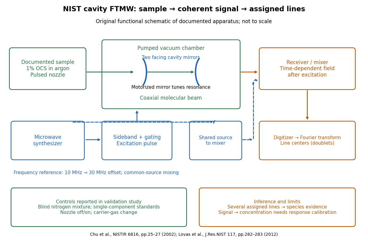
Original functional schematic of the NIST trace-gas FTMW validation experiment
. An original arrangement of the documented sample, cavity, excitation and readout functions; no published figure is copied. The frequency-reference branch summarizes the later portable electronics described in the NIST historical account. The sample fraction is a reported preparation, not a synthetic measured spectrum. Details.
The portable electronics used a common microwave source and a offset derived from a reference. Cavity tuning selects the accessible band; it does not independently calibrate the line's frequency. Absolute accuracy also requires a characterized reference and receiver offset.[ref]
Evolution of Microwave Spectroscopy at the National Bureau of Standards (NBS) and the National Institute of Standards and Technology (NIST) by F. J. Lovas and others. §5, printed pp. 282–283, Figure 20: source splitting, frequency reference, single-sideband modulation, mixer and digitizer
Reported controls included nozzle off/on, carrier-gas changes, and a blind nitrogen mixture. Assigned components were correctly identified. Single-component standards supplied preliminary concentration calibration; one standard per quantified component left response validation incomplete. Condensation and departure from thermal equilibrium in the nozzle were acknowledged limitations.[ref]
The Validation of Fourier-Transform Microwave Spectroscopy for Trace-Gas Analysis. printed pp. 26–27: nozzle/carrier comparison in Figure 6, blind mixture in Table II, one-standard calibration and nozzle-expansion limitations
The lesson is that rotational spectral line assignment and concentration inference answer different questions. Reproducible frequencies support molecular identity; converting signal size into concentration requires calibrated response under the same transfer and excitation conditions. The thermal absorption example above does not model a nozzle's nonequilibrium populations or the cavity's pulsed response.
Sepal Created 2026-10-14 Updated 2026-11-05
Petal Created 2026-10-14 Updated 2026-11-05
Carpel 2026-10-14
Quantifier Created 2026-10-14 Updated 2026-10-25
A quantifier binds a free variable in a first-order formula and specifies how its truth depends on elements of a first-order structure: universal quantification requires every element, while existential quantification requires at least one.
Empty and open feasible regions 2026-10-14
Adding an optimization constraint removes possibilities: if it permits a set , the new feasible region is . It can leave unchanged when all its members already satisfy the added restriction. For a fixed objective function, restricting the feasible set cannot lower a minimization problem's infimum. In the equality slice of a feasible triangle, it raises the attained value from to .
Instead add to the feasible triangle with a squared-distance objective. No point can have both and . The resulting feasible set is the empty set, so there is no feasible point and no optimizing decision. Under the extended-value convention for a minimization problem, its infimum is .[ref]
A nonempty feasible set can also lack an optimizing decision. With domain , minimize subject to the strict inequality . The feasible region is an open set. Its infimum is , approached by the feasible points , but is excluded. Every feasible point is beaten by , so no minimum is attained. Replacing by includes the missing optimum. Open feasible regions do not always prevent attainment: minimizing on the same open set attains value at . A useful sufficient condition is instead the extreme value theorem: a continuous objective function on a nonempty compact set attains its minimum.
Equality slice of a feasible triangle 2026-10-14
Keep the feasible triangle with a squared-distance objective, but add the equation . An equality requires an exact relation, whereas an inequality allows a range. Here the equality selects a line, and intersecting that line with the original feasible region leaves just the line segment from to :The lower bound comes from ; the upper bound comes from . This is a nonempty closed set even though it has empty interior in the plane. An equality can reduce the dimension of the allowed decisions without making the feasible region empty.
The old optimum violates the added equality. On the surviving line segment, the objective function isThe derivative shows that the unique global minimum is at , giving and value . The nearest point on the entire equality line would be , at with value , but it violates . Both the equality and the original inequalities must hold simultaneously.
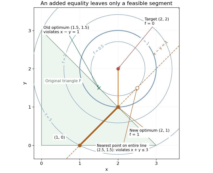
Equality slice of a feasible triangle: the allowed line segment ends at the optimum (2,1), while the nearest point on the entire line is infeasible
. Details. 
Use and to fix the multiplier sign convention in the optimization Lagrangian ; the Lagrange multipliers of and are again zero. At , Karush-Kuhn-Tucker conditions hold with and :The Lagrange multiplier of an equality has no nonnegativity restriction. For an independent global certificate, completing the square gives . On the feasible set, and , so , with equality exactly at .
Feasible triangle with a squared-distance objective Created 2026-10-14 Updated 2026-10-31
Take the decision domain and minimize the objective functionEach inequality permits a closed half-space; their intersection is the filled triangle with vertices , and , including its edges. The feasible region is a compact set and a convex set. The point is a feasible point, but its objective function value will not be best. Without the optimization constraints, the unique global minimum is at with value . That point is infeasible because .
The objective function is the squared Euclidean distance from . Its positive level sets are circles centered there. Expanding a circle from that center, the first contact with the feasible region is at , with objective function value . Thus the optimum is the Euclidean projection onto a convex set of the target . Squaring a nonnegative Euclidean distance preserves which point is nearest.[ref]
Convex Optimization by Stephen Boyd and Lieven Vandenberghe. §8.1.1, printed p. 398: squared Euclidean projection onto a polyhedron and half-space projection formula
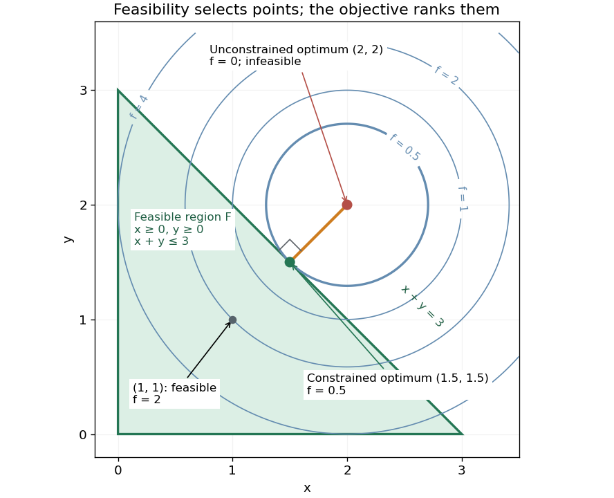
Feasible triangle with a squared-distance objective: the first attainable level set has value 0.5 at (1.5,1.5)
. Details. 
Here is a direct certificate, without relying on the picture. Put and . The objective function becomesEquality requires and , so the unique optimum is . At this point is an active constraint, while and are strict. An active constraint identifies a tight restriction at a specified point; it alone does not establish optimality. For example, has the same tight sum restriction but objective function value .
For a check using the Karush-Kuhn-Tucker conditions, write the inequalities as , , . Their Lagrange multipliers at the optimum are . The gradient equation isFeasibility, nonnegative Lagrange multipliers and complementary slackness also hold. With this strictly convex function and affine optimization constraints, the Karush-Kuhn-Tucker conditions certify the unique global minimum.[ref]
Convex Optimization by Stephen Boyd and Lieven Vandenberghe. §5.5.3, printed pp. 243–244, equation (5.49) and sufficiency for convex problems
Scanning Fabry–Pérot measurement 2026-10-14
An actual teaching experiment in LM-0300 Fabry Perot Spectrum Analyser by Walter Luhs, §§3.1.1–3.1.2, prepares a green laser beam by aligning it near and far along a rail, then centring back-reflected light from adjustable curved mirrors. An actuator using piezoelectricity moves one mirror. A screen first displays interference fringes; a focusing optical lens and photodiode then replace the viewing arrangement. The oscilloscope records the photodiode signal and the piezo drive reference on separate channels, using the latter as its trigger. Alignment and mirror separation are adjusted to suppress extra transverse normal modes; source temperature and drive electric current are controlled. Repeated peaks calibrate the scan using the appropriate free spectral range, and their spacing divided by their full width at half maximum estimates finesse.[ref]
This experiment uses a confocal curved-mirror cavity, whose repeated peak families can have spacing in air; it must not be calibrated blindly with the parallel-mirror . Extra transverse normal modes can mimic source features. A finite measured peak width bounds source sharpness only after instrumental broadening is considered; it does not determine the source's intrinsic width by itself.[ref]
LM-0300 Fabry Perot Spectrum Analyser by Walter Luhs. §3.1.2 p. 20: transverse modes, confocal calibration and source-linewidth inference
For an independent ideal scan calculation, hold a narrow laser wavelength fixed and vary the parallel-mirror gap at normal incidence. Advancing one resonance order requires . If changes uniformly over the measured interval, the time between repeated peaks divided by their full width at half maximum in time equals finesse. The cancellation of scan rate follows from : both peak spacing and peak width are divided by the same . It fails if the scan rate changes appreciably over that interval. A practical control in the University of Washington's motor-driven flat-mirror experiment is to check that successive peaks are equally spaced before using the time axis this way; its handout also warns that table strain and aggressive low-pass filtering alter the trace.[ref]
Fabry–Pérot etalon 2026-10-14
A Fabry–Pérot etalon fixes mirror separation in a Fabry–Pérot interferometer, selecting wavelengths through its transmission resonances.[ref]
Finesse 2026-10-14
The finesse of a Fabry–Pérot interferometer is its free spectral range divided by a transmission peak's full width at half maximum. Large finesse means a narrow accepted frequency interval compared with the spacing between repeated orders. Here half maximum means of the ideal unit peak, with zero detector background subtracted; it does not mean halfway between the transmission minimum and maximum.
Write for the coefficient multiplying in Fabry–Pérot transmission from multiple reflections. This coefficient is sometimes called the coefficient of finesse; it is not the finesse . About a resonance , put . Solving givesand, since one free spectral range advances the wave phase by ,These are exact for the ideal nondispersive model with constant and linear frequency dependence of . The inverse sine requires , or . At equality, neighbouring peaks merely touch half maximum at their shared minima: the nominal width is one full free spectral range and . Isolated half-maximum peaks require the strict inequality. Below this threshold the transmission never falls to , so this peak-width definition supplies no finesse; at the transmission is flat.
For large reflectivity, the small-angle approximation givesThis is a high-reflectivity approximation, not an identity for every . The original dimensionless examples below have exact full width at half maximum values obtained from the inverse sine formula.
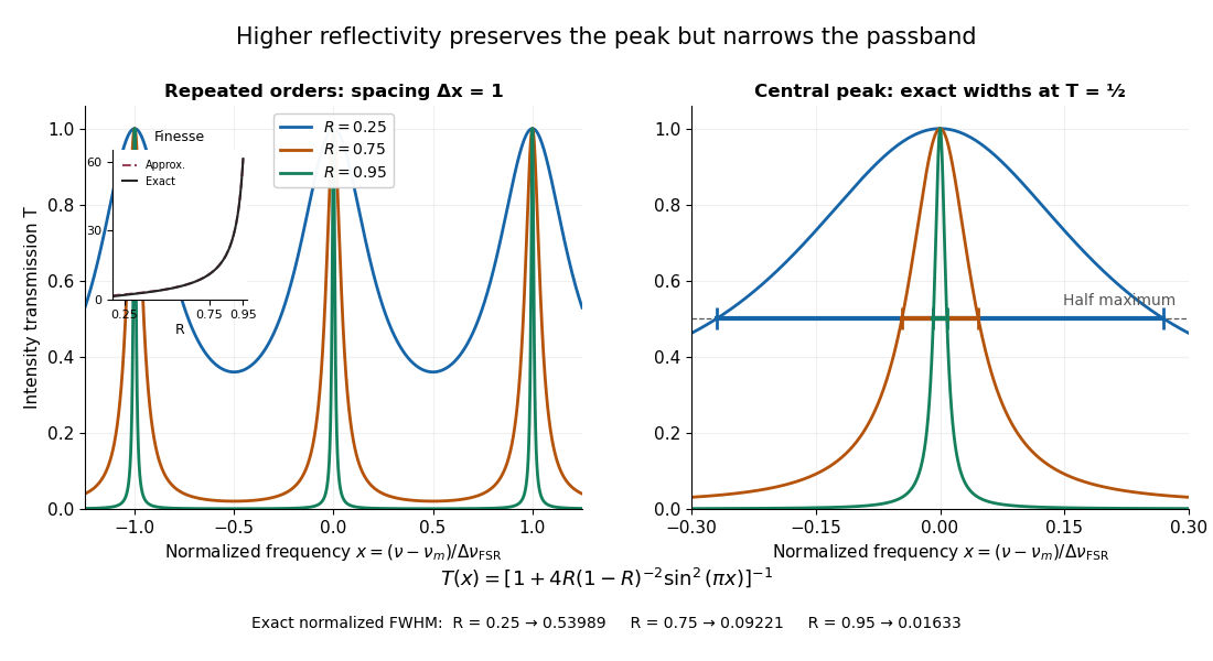
Increasing mirror reflectivity narrows Fabry–Pérot interferometer transmission peaks
. Original stipulated dimensionless model for , with and modulo . All curves peak at unity and repeat after . The second panel enlarges the central resonance; coloured segments at mark each exact full width at half maximum. The inset compares exact finesse with the high-reflectivity approximation. These are calculations, not measured scans. Details.
The beauty of the narrowing is visible directly in the geometric series: large preserves contributions from many round trips, so a small phase difference accumulates across many terms and spoils their addition. For the stipulated vacuum gap, gives an ideal full width at half maximum of about . This instrumental width is not a measured spectral line width. A real scan also depends on the source profile, accepted angles, mirror shape, alignment, and scan stability. The University of Washington handout separately discusses mirror-reflectivity, mirror-flatness, and detector-pinhole contributions; increasing alone cannot remove the others.[ref]
Fabry-Perot Interferometer, University of Washington Physics 331. Finesse discussion, equations (5)–(8), and §2.3 Determine the Finesse
Fabry–Pérot resonance spacing 2026-10-14
At normal incidence, with no optical dispersion and zero round-trip reflection wave phase modulo , the resonance condition in Fabry–Pérot transmission from multiple reflections isHere is frequency and is the speed of light in vacuum. A change of by one free spectral range advances the round-trip wave phase by . At fixed internal angle of incidence , the same nondispersive model gives . Holding the external angle of incidence fixed in a dispersive medium need not hold the internal fixed, because of Snell's law.
For stipulated and , the free spectral range is using . A frequency difference of is therefore . Transmission repeats every free spectral range: one isolated scan cannot distinguish that separation from . Independent knowledge of the optical spectrum, an additional filter, or a changed mirror separation is needed to assign orders.
Equal spacing in frequency does not imply equal spacing in wavelength. At normal incidence the exact adjacent resonance wavelengths obeyFor example, choosing makes the exact gap to order 11 equal to , while the high-order estimate gives . The approximation is already ten percent larger at order 10. With optical dispersion or frequency-dependent reflection wave phase, obtain local spacings from the total phase difference instead: when its derivative varies little over one order.
Fabry–Pérot transmission from multiple reflections Created 2026-10-14 Updated 2026-10-20
Consider two identical, lossless parallel mirrors with intensity reflectivity , separation , and a uniform transparent medium of refractive index . Fix one polarization of an electromagnetic wave and an internal angle of incidence measured from the mirror normal vector. Illuminate with a monochromatic wave having planar wavefronts; the emerging contributions must overlap coherently in the detected direction. Define using the same incident and exit media. Each mirror transmits a fraction of incident power. Its reflected wave amplitude has magnitude , so two internal specular reflections multiply the circulating complex amplitude by magnitude , not .
Let be the vacuum wavelength and choose the reflection wave phase convention in which the product of the two internal amplitude reflection coefficients is real and positive. The phase difference between successive transmitted contributions, evaluated on a common outgoing wavefront, isWith other mirror coatings or phase conventions, use the total , where is the sum of the two internal reflection wave phases. The stated resonance positions presume modulo ; a constant nonzero shifts them, while a frequency-dependent one can also change their spacing.
Why does the cosine appear rather than its reciprocal? Inside the gap, the extra two legs have optical path length . But the later emerging contribution starts farther along the mirror. Comparing both on one outgoing wavefront subtracts from that path difference, leaving . Equivalently, a plane wave's mirror-normal wavevector component is , so the round-trip wave phase is . The diagram uses the same medium outside and inside to show the common-wavefront subtraction directly; at a refracting exit interface, tangential wavevector matching in Snell's law supplies the same result.
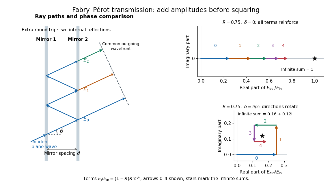

Absorb the common first-pass wave phase into the incident complex amplitude . Successive transmitted contributions are , , and so on. The superposition principle and the convergent geometric series giveThe last step expands the squared complex modulus as . This transmission profile is often called the Airy transmission function; it is distinct from the Airy disk, a diffraction image of a circular aperture. The University of Washington's lab handout gives the same transmission profile and distinguishes mirror reflectivity from other sources of peak broadening.[ref]
Fabry-Perot Interferometer, University of Washington Physics 331. Fabry-Perot Interferometer, theory equation (2), Finesse discussion, equations (4)–(8)
For an original example, set . At , the amplitudes add to , so . At , they alternate in sign and add to , so . At , the amplitude is and . Adding the individual intensities instead would give , independent of wave phase; that discards the wave interference responsible for the peaks.
In general the maximum is at , with integer , and the minimum is halfway between peaks. Perfect resonant transmission requires identical lossless mirrors, coherent illumination, and sufficient time to establish the steady field. Absorption, unequal mirror transmission, finite beams that fail to overlap, and fluctuations of can reduce it. The exactly reflecting case is excluded: no incident power enters through a perfectly reflecting mirror, and the resonant limit is singular.
The cotangent partial-fraction expansion gives, on ,The Bernoulli number generating function gives the same Laurent series in another form:The term cancels the separate ; the higher odd Bernoulli numbers vanish. Comparing Laurent coefficients therefore gives , which is the stated real formula because . The cotangent partial-fraction expansion justifies the convergent expansion before the coefficient comparison; a finite plot of partial sums alone would not prove the infinite identity.
Zeta series truncation error 2026-10-14
For a real exponent and a positive integer , the series truncation error in the defining Riemann zeta function series isThe integral comparison for the positive decreasing function gives the explicit boundsOn each unit interval, the area under lies between its endpoint heights. Summing from the first omitted term gives the lower integral from to infinity and the upper integral from to infinity. This uses positivity and monotonicity, not an assumption that the last computed term equals the remaining error.
At , the bounds are , whereas . The errors above fit both intervals. Merely looking at the eleventh term would give for squares, far smaller than the actual remaining .
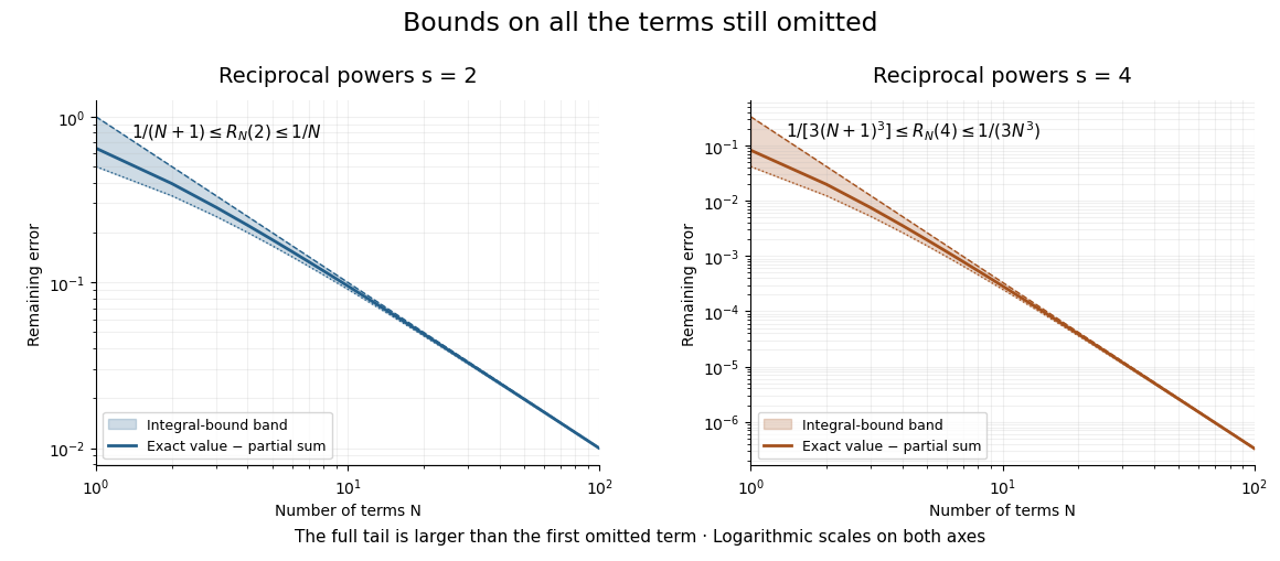

For a chosen absolute error target , the sufficient condition is , rounded upward to an integer. Thus requires by this bound for squares but only for fourth powers. This is a guarantee from an upper bound, not a claim that those are the smallest successful term counts.
Joule-Thomson effect 2026-10-14
The Joule-Thomson effect is the temperature response of a fluid flowing from higher to lower pressure through a valve or a plug of porous medium, when the throttle is insulated and the other steady-flow energy balance assumptions hold. Its equilibrium endpoints have equal specific enthalpy. The Joule-Thomson coefficient determines whether a small drop cools or warms; cooling is not universal.
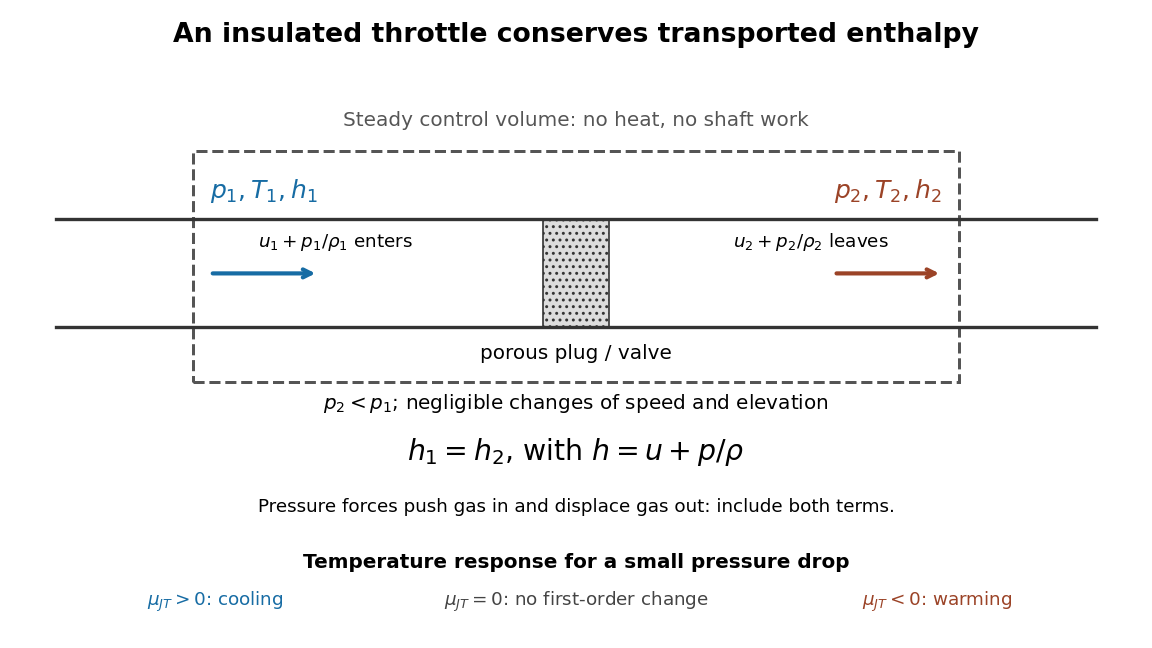
Enthalpy accounting for an insulated Joule-Thomson effect throttle
. Original schematic of the steady-flow energy balance, with denoting internal energy per unit mass. The arrows include inlet and outlet pressure work. The reduced balance requires negligible bulk kinetic energy and potential energy changes. No particular apparatus or measured temperature drop is depicted. Details.
A useful contrast is between three insulated expansions. In free expansion of a gas-only closed system into a vacuum, no external work occurs and ; an ideal gas returns to its initial equilibrium temperature. In a throttle, continuous flow carries pressure work across the boundary and preserves specific enthalpy under the stated assumptions; an ideal gas again has no endpoint temperature change. In a reversible adiabatic expansion of a loaded closed system, the gas supplies work, loses internal energy and cools, even if it is an ideal gas. That process preserves entropy; throttling generally produces entropy. For a small constant-enthalpy step, gives when and . This equilibrium comparison computes endpoint entropy differences without supplying a reversible path through the plug.
The effect is useful in refrigerators because an appropriately prepared real gas can cool while passing through a simple valve. The inlet must lie in a suitable positive-Joule-Thomson coefficient region. The Joule-Thomson inversion curve makes that requirement precise; a pressure drop by itself is not a guarantee of refrigeration.
Steady-flow energy balance 2026-10-14
For steady flow through a fixed control volume with one inlet and one outlet, the first law of thermodynamics and conservation of mass giveHere is the mass flow rate, incoming heat per unit time, outgoing non-flow work per unit time, the flow speed, elevation and gravitational acceleration. The specific enthalpy includes both the transported internal energy per unit mass and the pressure work needed to push volume through the boundary; is mass density. The inlet supplies that pressure work, while the outlet consumes it to displace the downstream fluid.[ref]
Thermodynamics and Propulsion. §2.5.1–2.5.2, equation 2.11: mass conservation, transported enthalpy and the steady-flow energy equation
For an insulated stationary throttle, require negligible heat transfer, no shaft or other non-flow work, and negligible changes in bulk kinetic energy and gravitational potential energy. Then . With unchanged composition this is also equality of molar enthalpy. The upstream and downstream states must admit equilibrium pressure, temperature and property values, although the constriction itself is irreversible and can be far from thermodynamic equilibrium. Start-up storage of energy in the walls and fluid, heat leakage, or a large outlet speed invalidates the reduced balance. A nozzle can convert specific enthalpy into bulk kinetic energy even when it is insulated.
The same accounting for a fixed transported amount is , hence . This explains why dropping the two pressure work terms would give the wrong conserved quantity.[ref]
Isenthalpic process 2026-10-14
An isenthalpic process preserves enthalpy for a fixed amount of material, or preserves specific enthalpy between inlet and outlet when comparing a flowing fluid of fixed composition. It need not preserve temperature or entropy. An insulated throttle satisfying the steady-flow energy balance assumptions is an important example.
Molar enthalpy Created 2026-10-14 Updated 2026-10-20
Molar enthalpy is enthalpy per amount of substance , measured in . With and molar volume , . Its fixed-pressure temperature derivative is the corresponding molar heat capacity , at fixed composition.
Lock-in amplifier Created 2026-10-14 Updated 2026-10-18
A lock-in amplifier measures the component of an input signal synchronized with a reference at a chosen frequency. It multiplies the input by a reference sinusoid, then uses a low-pass filter to retain the slowly varying product. Two references in phase quadrature recover both amplitude and phase difference. A shared timing source keeps the relative wave phase stable: this is coherent detection.[ref]
Model SR830 DSP Lock-In Amplifier manual by Stanford Research Systems. Model SR830 DSP Lock-In Amplifier manual, revision 2.5, printed pp. 3-1–3-2: multiplication, filtering, reference locking and dual-phase detection
The useful trick is to move the wanted frequency to zero before averaging. An electronic amplifier alone enlarges both the wanted signal and unwanted noise; a lock-in amplifier instead selects a component by its timing. A photodiode's electric current can first be converted to an electric potential difference, so the same calculation can measure weak modulated light. The chopped-light lock-in experiment makes this selection tangible.
There are unlisted articles, also show them or only show them.