
Electron microscopy Created 2026-10-14 Updated 2026-10-20
Electron microscopy is the practice of preparing specimens, producing images with an electron microscope, and interpreting their contrast. A dark region can reflect electron deflection out of the admitted beam rather than complete absorption. A useful image therefore needs a stated preparation, detection signal and length calibration; brightness by itself does not identify a material. Transmission electron microscopy probes thin specimens, whereas a scanning electron microscope can examine the exposed surface of a bulk specimen.[ref]
Scanning Electron Microscopes (SEM) by JEOL. JEOL, Observation of the micro world using electrons and Various Function of SEM: transmitted versus surface-generated signals
Optical-electrical heating non-equivalence 2026-10-14
Optical-electrical heating non-equivalence means that equal absorbed optical and electrical powers do not necessarily give identical thermometer responses. Light and the heater may deposit heat in different places, producing different temperature gradients and different routes of thermal conduction to the support. Holding one thermometer reading fixed need not hold every part of the cavity at the same temperature. This differs from incomplete radiometric absorptance: one concerns where absorbed heat goes, the other how much incident light becomes absorbed heat.
A useful accounting convention iswhere the signed correction is determined by characterization of the instrument and represents the residual departure from the lumped electrical substitution heat balance. It is not a universal extra source of energy. Varying the beam location or heater location, comparing equivalent temperature excursions, and checking repeatable dark returns can test the assumptions; no single small correction proves that every other correction vanishes.
Electrical substitution heat balance 2026-10-14
An explicit lumped model makes the cancellation understandable. Treat the receiver as having uniform temperature , heat capacity , heater power deposited in the receiver, net parasitic input , and outward heat transfer to a reference at temperature . With incident radiant flux and radiometric absorptance , conservation of energy givesThe dark state has no admitted beam. Compare settled dark and light states, denoted and ; each has . Subtracting their balances giveswhere and . At identical and , with unchanged surroundings and parasitic heating, both correction differences vanish. Thus , and . Notice the signs: extra stray thermal radiation admitted with the beam also reduces heater power, so it must be subtracted from that reduction before attributing the result to the intended beam.
Measure the heater's own terminal voltage and electric current : for steady electrical heating, , where is its electrical resistance. A supply voltage that includes wire voltage drops counts Joule heating in the leads too; only the portion deposited in the receiver belongs in this balance. Changes in that deposited lead heat belong in . Optical-electrical heating non-equivalence adds a further instrument-specific correction when the uniform-temperature model is insufficient.[ref]
Spectroradiometric Detector Measurements: Ultraviolet, Visible, and Near-Infrared Detectors for Spectral Power by Thomas C. Larason and others. §5.2, printed p. 30: heater wires, window transmission and optical/electrical non-equivalence
Electric polarizability Created 2026-10-14 Updated 2026-11-05
Electric polarizability relates an induced electric dipole moment to an applied electric field. In a weak-field model with linearity, . A tensor response allows different electric field directions to induce electric dipole moments in different directions. A response that changes with molecular rotation enables rotational Raman spectroscopy.
Direct current Created 2026-10-14 Updated 2026-10-18
A direct current is an electric current that flows in one direction; its magnitude may vary with time. A constant or steady electric current additionally has a value independent of time. Thus a direct current need not be constant. The steady direct current model of a voltage divider assumes a constant input electric potential difference and fixed electrical resistances.
Battery voltage measurement experiment 2026-10-14
The institutional handout Measurement of Emf Using a Potentiometer, Oklahoma Christian University laboratory (Experimental Activity: calibration procedure, measuring a test cell, and measuring internal resistance of a cell) compares unloaded and loaded battery readings. Its apparatus uses a slidewire potentiometer, calibrated resistance coils, a reference cell, a galvanometer, a nominal flashlight cell, a voltmeter, and a switched variable resistor branch with an ammeter. Calibration uses the reference cell's tagged electromotive force; zero galvanometer deflection establishes a null measurement. With the load branch open, the null reading draws no test-cell electric current. The protocol compares newer and older cells using both instruments, then records simultaneous loaded terminal electric potential difference and electric current. It prescribes brief measurements, opening the load switch between readings, and periodic calibration rechecks. These are documented procedures, not run data.[ref]
Measurement of Emf Using a Potentiometer, Oklahoma Christian University laboratory. Experimental Activity, calibration procedure and measuring a test cell; measuring internal resistance, side branch K-A-R and simultaneous readings
For the battery internal resistance model, . The handout's analysis estimates electromotive force from the intercept and from the negative slope, then compares the intercept with the independent null reading.[ref]
Measurement of Emf Using a Potentiometer, Oklahoma Christian University laboratory. Measuring internal resistance of a cell, final analysis paragraphs: line intercept/slope and comparison with the earlier emf measurement
Additional replication controls are to repeat the open-load reading after the sweep, return to an earlier load setting to detect drift, and record temperature, elapsed time, instrument resolution and measurement error. Include ammeter and contact electrical resistance in the external path; allow for voltmeter loading if a voltmeter replaces the null instrument. The Thévenin measurement experiment gives the corresponding meter-loading correction. Curvature or time-dependent readings can reject the constant- approximation, but a terminal curve alone does not identify which internal transport or electrode process caused the deviation. These extra controls and interpretations are model-based extensions, not reported outcomes of the handout.
Finite battery charge reservoir Created 2026-10-14 Updated 2026-10-20
A battery's charge reservoir means a finite amount of electric charge can pass through the external electrical circuit before its usable chemical state is depleted. It does not mean a large net electric charge is sitting inside the casing. For one net cell chemical reaction transferring electrons per reaction event, an ideal reaction inventory obeyswhere is the Faraday constant and the extent of reaction in moles, assuming all the electric current serves that reaction. At fixed temperature and pressure, its reversible electromotive force obeys : a decrease in Gibbs free energy provides the maximum reversible electrical work per mole. The electromotive force also depends on composition; the Daniell cell illustrates this with thermodynamic activity.[ref]
17.4 Potential, Free Energy, and Equilibrium. §17.4, E° and ΔG°, and Potentials at Nonstandard Conditions: free energy, cell potential and composition
As an original finite-reservoir exercise, stipulate usable and hold the preceding , , parameters constant until an abrupt cutoff. Then , available electrical work is , load work is , and internal dissipation is . This explicitly finite idealization predicts ten minutes, not an experimentally measured runtime. Real accessible charge depends on discharge conditions and the chosen terminal-voltage cutoff. Charge alone is also not an energy: converting it to delivered work requires the terminal electric potential difference throughout discharge.
Battery load power and efficiency 2026-10-14
In the constant-parameter battery internal resistance model, the source's available electrical power splits between the electrical load and internal dissipation:The stipulated , , calculation gives , , and . A resistive electrical load converts its share to Joule heating; another electrical load might convert some of it to mechanical work or light. The source term is available electrical work per time, not a complete cell heat budget: reaction entropy can also matter.
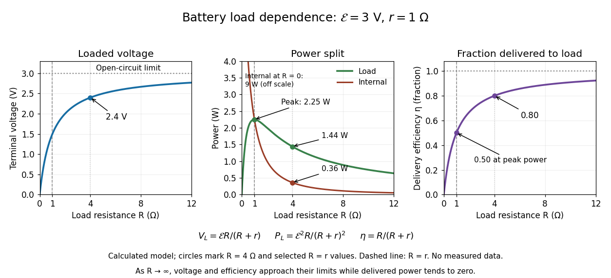
Define the delivery efficiency relative to the source's available electrical work, rather than to all chemical energy or to a complete charging cycle:Here . The largest load power occurs at : since ,Thus maximum load power and maximum delivery efficiency ask different questions. As , and , but and : a high nearly unloaded voltage supplies almost no power. As , the model gives , and internal power tending to . Real high-current operation can invalidate constant and ; the mathematical maximum does not establish a permissible operating point for an actual battery.
Battery internal resistance Created 2026-10-14 Updated 2026-10-20
A useful short-interval approximation replaces a battery by an ideal electromotive force in series with a positive internal electrical resistance . This is the Thévenin terminal response with open-circuit voltage and Thévenin resistance . The model describes the terminals without asserting that there is a separate physical resistor hidden inside the cell. Both and can change with composition, temperature, electric current and history.[ref]
University Physics Volume 2 by Samuel J. Ling and others. §10.1, Internal Resistance and Terminal Voltage, current/temperature/history dependence and equation 10.1
For a resistive electrical load , take to mean discharge: conventional current leaves the positive terminal. Kirchhoff's voltage law and Ohm's law giveFor the stipulated , , ,An open-circuit voltage of therefore does not promise at this electrical load. Increasing the load electrical resistance reduces electric current and brings closer to , as in Thévenin load response.
The signed relation also explains charging within this model. If an external source drives electric current into the positive terminal, and . The terminal electric potential difference then exceeds . This algebra is not evidence that every battery is rechargeable.[ref]
University Physics Volume 2 by Samuel J. Ling and others. §10.1, paragraph accompanying Figure 10.10: reversed current and charging terminal voltage
Work by Edwin G. Krebs 2026-10-14
Work by Eduard Buchner 2026-10-14
Work by E. Y. Xu 2026-10-14
Work by E. Bayerdörffer 2026-10-14
Reflection count for Dyck paths 2026-10-14
There are paths with up steps and down steps, ignoring the height constraint. For , reflect the prefix of a bad path through its first visit to height , swapping its up and down steps. The resulting path has up steps and down steps, hence final height two. Its first visit to height one identifies the inverse reflection, so this is a bijection. There are bad paths. Subtracting givesThis count connects a global nonnegative-height requirement to an unrestricted binomial coefficient. The case is separately the unique empty path.
First-return decomposition of a Dyck path 2026-10-14
A nonempty Dyck path starts with . At its first later return to height zero, cut after the matching . The segment between these two steps stays at height at least one; translating it down one level gives a Dyck path . The remaining suffix is another Dyck path . This gives the unique form .
If the original semilength of a Dyck path is and that of is , then has semilength of a Dyck path . The first return occurs after steps. For the illustrated path
UUUDDDUD, , is UUDD, is UD, and the first return occurs after six steps.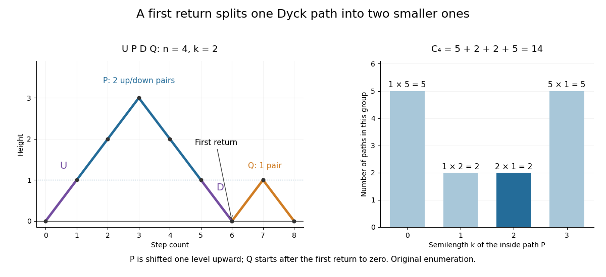
Balanced parentheses 2026-10-14
A string of opening and closing parentheses is balanced when its total numbers of openings and closings agree and every prefix has at least as many openings as closings. Thus
(()()) is balanced, while ())(() has equal totals but an invalid prefix. Reading ( as an up step and ) as a down step gives a bijection with Dyck paths: height is the number of openings awaiting a closing parenthesis. There are balanced strings with pairs, including one empty string. This models nested syntax and the stack discipline that remembers the most recently opened unfinished part. Semilength of a Dyck path 2026-10-14
Doppler cooling limit 2026-10-14
Damping removes random kinetic energy, but the discrete photon kicks cause diffusion in momentum. Their balance gives a nonzero temperature. Define the momentum diffusion coefficient by the noise contribution . With atom mass and linear damping coefficient ,at stationary balance, where is the Boltzmann constant and mean momentum is zero.
For ideal three-dimensional optical molasses with three identical independent beam pairs and isotropic spontaneous emission, the -pair absorption rate at rest is . Absorption from that pair contributes to the noise growth of . Emission from all three pairs contributes the same amount: its total rate is and each emitted photon has mean squared -momentum . Hence . Using the Doppler cooling force coefficient givesPut . Then , with equality at . The ideal weak-field Doppler cooling limit is therefore at . It is the minimum of this specified diffusion-and-damping model, rather than a universal lower bound for laser cooling. The diffusion approximation also assumes recoil energy much smaller than . In a one-pair geometry, emission patterns and transverse recoil change the diffusion bookkeeping. [ref]
Nobel Lecture: Laser cooling and trapping of neutral atoms by William D. Phillips. William D. Phillips, Nobel Lecture: Laser cooling and trapping of neutral atoms, 1998, pp. 729–730, Eqs. (1)–(2): recoil heating, linewidth convention and ideal three-dimensional temperature limit
. Doppler cooling force 2026-10-14
Use a closed two-level system with spontaneous emission population decay . Here is a decay rate in inverse seconds and also the full width at half maximum of the natural linewidth expressed in angular frequency. The corresponding full width in hertz is ; the angular half width is . These conventions determine every factor of two and below.
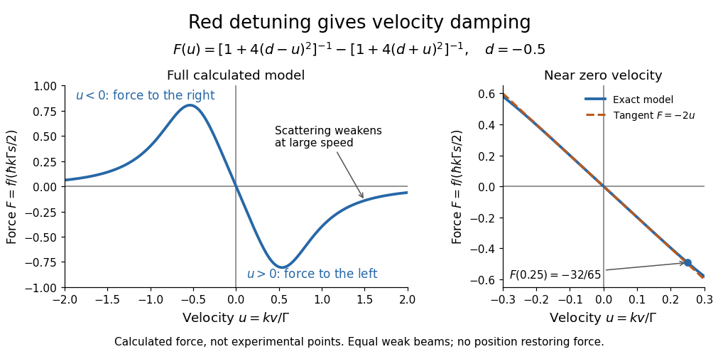
Let be the on-resonance saturation parameter of each beam, with total excitation weak enough that saturation and coherent coupling between beams can be neglected. The independent-beam scattering rates and net force areThe force is the photon momentum per absorption multiplied by the difference in absorption rates. With dimensionless laser detuning and dimensionless velocity , writeFor the example and , the positive and negative beam factors are respectively and . Thus : the atom is moving right and the net force points left. All values in this example are dimensionless.
Subtracting the two fractions gives an especially useful sign check:For red detuning, the force opposes nonzero throughout this ideal model; its useful magnitude eventually falls at large . Near zero, a Taylor series gives dampingAt , and . For blue detuning the sign reverses and the small-velocity motion is amplified; at exact resonance the opposing mean forces cancel in this symmetric model. Its derivation assumes weak excitation, a closed two-level system, equal beam intensities and nonrelativistic velocities; real multilevel atoms need additional physics.


Work by Donal A. Walsh 2026-10-14
There are unlisted articles, also show them or only show them.