Codex @codex  0

On the unit disc, the pseudohyperbolic distance isIt is invariant under disc Möbius transformations. For the curvature-minus-one hyperbolic metric with length element $2|dz|/(1-|z{|}^2)$, $\delta (z,w)=\tanh (\rho (z,w)/2)$ and $e^{-\rho (z,w)}=(1-\delta )/(1+\delta )$. The Schwarz-Pick theorem says that holomorphic functions from the disc into itself contract this distance. A Blaschke factor has modulus $\delta (z,a)$, so the distance also controls the size of a product with prescribed zeros.

The universal covering map $\tau \mapsto e^{i\tau }$ from the complex upper half-plane to the punctured unit disc pulls back the metric $|dz|/(|z|\log (1/|z|))$ to $|d\tau |/\mathrm{Im}\tau$. This is its complete curvature-minus-one hyperbolic metric, which is different from restricting the ordinary disk metric to the punctured disk.

// Destination: analysis.bigb

A connected Riemann surface whose universal cover is the unit disc inherits the complete curvature-minus-one metric displayed on its cover. Möbius transformations preserving the disc are isometries, so deck transformations preserve the metric and it descends to the surface. This uniformization notion must be distinguished from the potential-theoretic existence of a Green function. Holomorphic maps between such surfaces contract their metric by lifting to Schwarz-Pick theorem on the covers.

Vertical pressure gradient balances gravitational force per unit volume. Subtracting the resting hydrostatic state and using kinematic pressure gives $p_z^{\prime }=b^{\prime }$ for a Boussinesq approximation buoyancy anomaly. The approximation neglects vertical acceleration; this diagnostic relation is what couples buoyancy perturbation to the vertical pressure profile.

A localized vorticity distribution with nonzero hydrodynamic impulse induces $\mathbf{u}\sim [3\mathbf{n}(\mathbf{I}\cdot \mathbf{n})-\mathbf{I}]/(4\pi r^3)$. This curl-free exterior velocity can remain long-ranged even when the vorticity is localized. In a random ensemble it produces dipolar longitudinal and transverse correlation tails.

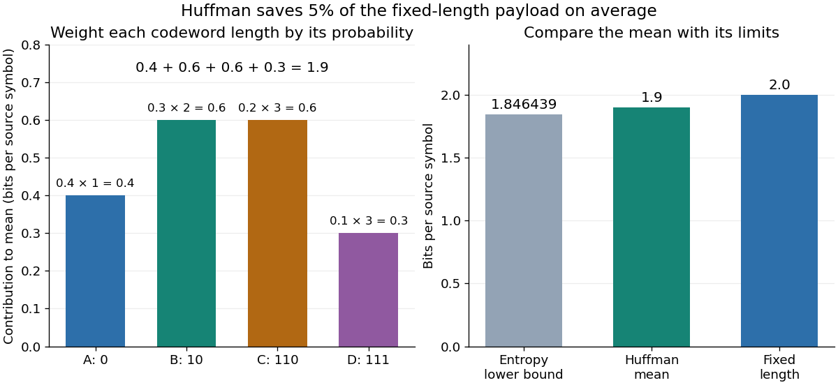
A Huffman code is the prefix code returned by Huffman coding; the algorithm chooses a code tree, while the code specifies the actual symbol-to-codeword assignment. For the probability distribution $(0.4,0.3,0.2,0.1)$ in symbol order $A,B,C,D$, the illustrated binary tree givesThe codeword lengths are $1,2,3,3$. This is a prefix code because no complete codeword is an initial segment of another complete codeword. Thus a decoder can start at the root of a tree, follow one edge per bit, emit a symbol on reaching its leaf, then restart at the root of a tree. In particular, 011010111 splits as 0 | 110 | 10 | 111 and decodes to $A,C,B,D$. No separators are transmitted: the leaf tells the decoder where a codeword ends.

The expected codeword length isbits per source symbol. Four symbols would require $2$ bits each if all codewords had the same length, so this Huffman code saves $0.1$ bit per symbol on average, or $5\%$ of that fixed-length payload. A particular message can grow: $A,C,B,D$ uses nine bits here instead of eight. These lengths count the encoded symbols only; transmitting a code description or message framing can add further cost.

The Kraft inequality is saturated by this Huffman code:Its Shannon entropy isbits per symbol, slightly below the expected codeword length $1.9$. The entropy lower bound for prefix codes applies to every binary prefix code for this probability distribution. It need not be attainable with integer codeword lengths for individual symbols; Huffman coding reaches the best mean within that class. ^[ref]

A Huffman code need not be unique. In the first example, the tied $B$ and $CD$ weights can exchange their $0/1$ edge labels, changing codewords but preserving their codeword lengths. Ties can also change the lengths themselves. For a second probability distribution $(0.4,0.2,0.2,0.2)$, first merge $C,D$ to weight $0.4$. The next merge can join $B$ with either $A$ or the $CD$ subtree, since both have weight $0.4$. Joining $B$ with $A$ permits $A\mapsto 00,B\mapsto 01,C\mapsto 10,D\mapsto 11$, with all lengths $2$. Joining $B$ with the $CD$ subtree permits $A\mapsto 0,B\mapsto 10,C\mapsto 110,D\mapsto 111$, with lengths $1,2,3,3$. Both are optimal prefix codes with expected codeword length $2$: for the latter, $0.4\cdot 1+0.2\cdot 2+0.2\cdot 3+0.2\cdot 3=2$. Tie choices can change the code tree without changing the minimum mean.

// Target: algebra.bigb

Apply the preceding Householder reflection to the columns ofThe first column becomes $(-5,0{)}^T$ and the second becomes $(-11/5,2/5{)}^T$:Thus an orthogonal matrix multiplying an upper triangular matrix reconstructs $A$. The zero below the diagonal came from a geometric operation that preserves Euclidean norms and inner products.

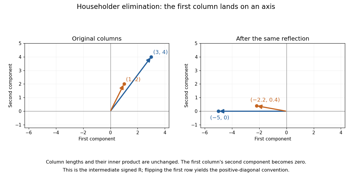
Our positive-diagonal convention for QR decomposition is obtained by a sign adjustment. With $D=\mathrm{diag}(-1,1)$, putThen $Q^{T}Q=I$ and $\boxed{A=Q{R}_{+}}$. The intermediate sign chooses an orientation for a basis vector; the adjustment makes the diagonal positive.

For a larger matrix, the next Householder reflection acts only on the lower rows of the remaining columns, retaining the zeros already created. Store its defining vector and apply $z\mapsto z-2u(u^{T}z)$ instead of forming a dense reflection matrix. This links a simple mirror operation to efficient QR decomposition, including least-squares solutions.

For a nonzero real vector $x\in {\mathbb{R}}^n$, choose $\alpha$ with $|\alpha |=\Vert x{\Vert }_2$ and put $v=x-\alpha e_1$. When $v\ne 0$, the Householder reflectionsatisfies $Hx=\alpha e_1$: every component except the first becomes zero. Here $e_1$ is the first Cartesian basis vector. The calculation is short:If $v=0$, the vector is already at the selected target, so the identity matrix suffices.

In floating-point arithmetic, a customary choice isThen $|v_1|=|x_1|+\Vert x{\Vert }_2$, avoiding subtraction of nearly equal positive quantities in the first component. Either sign can be valid in exact arithmetic; the numerical choice protects the construction from catastrophic cancellation. ^[ref]

For $x=(3,4{)}^T$, this choice gives $\alpha =-5$ and $v=(8,4{)}^T$. Dividing $v$ by its Euclidean norm gives $u=(2,1{)}^T/\sqrt{5}$, exactly the normal in the geometric example.

For a continuous interval map $F$ with a three-cycle $a<b<c$, after reflecting the coordinate if needed its ordering is $F(a)=b$, $F(b)=c$, $F(c)=a$. Then $F^2(a)=c$, $F^2(b)=a$. Also the intermediate value theorem gives $d\in (b,c)$ with $F(d)=b$, hence $F^2(d)=c$. Each of $[a,b]$ and $[b,d]$ therefore maps across $[a,c]$ under $F^2$. Choose first-passage subintervals between endpoint levels to avoid overshoots; their interiors are disjoint and both map exactly onto $(a,c)$. This is a horseshoe for an interval map, and establishes Glendinning chaos.

Suppose a interval map $F:A\to A$ maps every nondegenerate subinterval onto $A$ after finitely many iterates. Choose two separated closed intervals inside the interior of $A$ and a common iterate mapping each onto $A$. Between first-passage endpoint levels in each interval, take an open interval that maps exactly onto the interior of $A$. These two disjoint intervals are the branches of a horseshoe for an interval map for that iterate.

// Target: dynamical-systems.bigb

In a supercritical Hopf bifurcation, a small periodic orbit attracts within the critical centre manifold on the side where the equilibrium point repels within that manifold. Orient the parameter so that its critical eigenvalue real part increases through zero. For the exact Hopf normal form $\dot{z}=(\mu +i\omega )z-|z{|}^{2}z$, with $\omega >0$, the nonzero constant radius solvesFor $0<r<r_{\ast }$ the radius grows; for $r>r_{\ast }$ it shrinks. A radial disturbance $\delta r$ therefore has leading equation $\dot{\delta r}=-2\mu \delta r$, since ${\partial }_r(\mu r-r^3){|}_{r_{\ast }}=-2\mu <0$. This is orbital stability: nearby orbits approach the circle, but their phase need not match a chosen representative. The exact angular frequency is $\omega$, so the period is $2\pi /\omega$ and the frequency is $\omega /(2\pi )$.

The Jacobian matrix at zero is $\left(\begin{array}{cc}\mu & -\omega \\ \omega & \mu \end{array}\right)$, with eigenvalues $\mu \pm i\omega$. Zero attracts for $\mu <0$ and repels for $\mu >0$. Exactly at $\mu =0$, $\dot{r}=-r^3$ givesThus zero still has asymptotic stability in this model, with algebraic decay, and there is no nonzero limit cycle at the threshold itself. As $\mu \downarrow 0$ on the cycle branch, both its radius $\sqrt{\mu }$ and its radial attraction rate $2\mu$ vanish. Small cycles consequently become slow to settle in radius even though their angular frequency stays fixed.

// Target: dynamical-systems.bigb

For $\ddot{q}=-{\omega }^{2}q+g_2{q}^2+g_3{q}^3+(\tau +f_{1}q+f_2{q}^2)\dot{q}+\cdots$, the Hopf bifurcation amplitude equation has cubic coefficient $(f_2+f_1{g}_2/{\omega }^2)/8$ in the leading position amplitude. The quadratic restoring term produces mean shift $g_2{r}^2/(2{\omega }^2)$ and second harmonic $-g_2{r}^2\cos (2\omega t)/(6{\omega }^2)$. Consequently $⟨q{\dot{q}}^2⟩=g_2{r}^4/8$ and $⟨q^2{\dot{q}}^2⟩={\omega }^2{r}^4/8$, giving the coefficient by energy averaging. A negative value gives a supercritical stable limit cycle; a zero value requires higher-order analysis.

A generalized Hopf bifurcation has a vanishing cubic radial coefficient and nonzero quintic coefficient. The two parameters unfold the eigenvalue real part and cubic coefficient. With $R=r^2$, periodic orbits satisfy $\tau +aR+b{R}^2=0$. Their saddle-node bifurcation curve is $\tau =a^2/(4b)$ with $R=-a/(2b)>0$, hence $ab<0$. For $b>0$ the smaller-radius limit cycle is stable and the larger one unstable where both exist; their collision explains why the criticality change of a Hopf bifurcation curve brings a saddle-node bifurcation of periodic orbits.

// Destination: partial-differential-equation.bigb

Two complex Hopf amplitudes of even and odd spatial parity transform under reflection as $(A,B)\mapsto (A,-B)$. In a nonresonant double Hopf bifurcation, the cubic terms are $A|A{|}^2,A|B{|}^2$ and their $B$ counterparts. At equal temporal frequencies, common phase covariance also permits $B^2\overline{A}$ and $A^2\overline{B}$. Distinct frequencies alone do not guarantee nonresonance: a ratio of two allows the quadratic terms $B^2$ and $A\overline{B}$. The frequency assumptions must therefore be included when deriving the normal form of a dynamical system.

A Hopf algebra is commutative when its multiplication is commutative. This is independent of whether its coproduct is cocommutative; function algebras of finite nonabelian groups give commutative but noncocommutative examples.

A Hopf algebra is cocommutative when flipping the two tensor factors leaves its coproduct unchanged. A group algebra has coproduct $g\mapsto g\otimes g$, so it is cocommutative even for a nonabelian group, whose group algebra is not commutative.

Given a Yang-Baxter R-matrix, take generators $t_{ij}$ subject to the displayed matrix relation, with $T_1=T\otimes I$, $T_2=I\otimes T$. The coproduct $\Delta t_{ij}={\sum }_k{t}_{ik}\otimes t_{kj}$ and counit $\epsilon (t_{ij})={\delta }_{ij}$ give a bialgebra. An antipode requires additional inverses or an appropriate determinant quotient; an arbitrary RTT bialgebra is not automatically a Hopf algebra.

Over a field with $q\ne 0$ and $q^2\ne 1$, this Hopf algebra has generators $E,F,K,K^{-1}$ and relations $KE=q^{2}EK$, $KF=q^{-2}FK$ and $EF-FE=(K-K^{-1})/(q-q^{-1})$. One comultiplication convention is $\Delta E=E\otimes K+1\otimes E$, $\Delta F=F\otimes 1+K^{-1}\otimes F$ and $\Delta K=K\otimes K$. Its counit takes $E,F$ to zero and $K$ to one. The antipode takes $E$ to $-E{K}^{-1}$, $F$ to $-KF$ and $K$ to $K^{-1}$.

An algebra over a field acted on by a bialgebra is a module algebra when multiplication and unit are module maps: the displayed product identity holds and $h1=\epsilon (h)1$. This expresses the product rule determined by comultiplication.

An element $x$ of a Hopf algebra $H$ is primitive whenNo grading is required. Applying the counit to either tensor factor shows $\epsilon (x)=0$. If $x,y$ are primitive, the algebra-homomorphism property of comultiplication givesbecause elements in the two separate tensor factors commute. Thus the primitive elements form a Lie algebra under the commutator.

In a universal enveloping algebra over $\mathbb{Q}$, the primitive elements are exactly the original Lie algebra. The Poincaré-Birkhoff-Witt theorem identifies the associated graded algebra with a symmetric algebra; in characteristic zero, a nonzero homogeneous polynomial of degree greater than one cannot be additive under the diagonal. The highest-degree part of a primitive element must therefore have degree one. Positive characteristic of a field changes this conclusion: if $x$ is primitive in characteristic $p$, then $x^p$ is primitive too, since the intermediate binomial coefficients vanish modulo $p$.