
Sensible heat Created 2026-10-14 Updated 2026-10-20
Sensible heat is transferred heat associated with a temperature change within a single thermodynamic phase. By contrast, latent heat can change the phase fraction while the temperature stays fixed during equilibrium phase coexistence. Neither name denotes an additional stored substance: both describe how transferred heat participates in a process.
For fixed mass and composition, use the heat capacity appropriate to the heating constraint. Under the quasistatic process assumptions in heat capacity, with only pressure-volume work and unchanged bulk kinetic energy and potential energy, fixed-pressure heating givesHere is specific heat capacity at constant pressure; fixed-volume heating instead uses specific heat capacity at constant volume . A cooling step has negative with the sign convention in heat. A temperature difference has the same numerical value in units of the kelvin or degree Celsius. The integral follows by adding the small transfers , rather than assuming a constant heat capacity.
As a stylized ice-to-water example for a fixed-composition closed system at fixed pressure , take , an initial temperature of , melting at , and a final temperature of . Assume constant specific heat capacity at constant pressure values and , and latent heat of fusion . These are stipulated, rounded model values; ignore the container and heat losses, retain all the material, and assume only pressure-volume work under the quasistatic process conditions above. The three steps areOnly the first and third terms are sensible heat; the middle term is latent heat. The plateau begins after and ends after of total supplied heat. At total input, half the mass is liquid water and the temperature remains . The equilibrium phase transition temperature depends on pressure; this example stipulates a single fixed pressure. [ref]
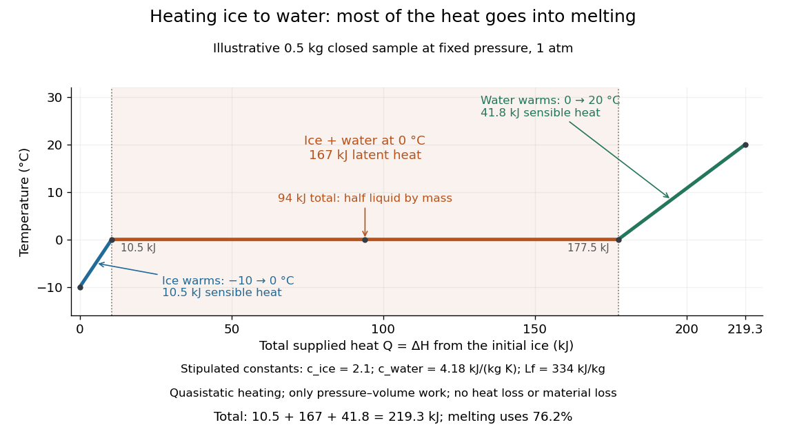

This split makes heating budgets easy to interpret: melting consumes of the supplied heat in this model despite causing no temperature rise. Within either single thermodynamic phase, the heating curve slope is ; a larger heat capacity makes the slope shallower. A flat interval represents changing phase fraction, so it cannot be modeled by applying across the phase transition. The complementary constructed example in latent heat tracks that phase fraction explicitly.
Completely regular Hausdorff space 2026-10-14
A Hausdorff space is completely regular if a point outside a closed set can be separated from by a continuous function with and . These functions determine the original topology: for any neighborhood of , choose to obtain . This is exactly the point-separation property needed for the evaluation embedding into the weak-star dual of bounded continuous functions.
Hartogs number 2026-10-14
The least ordinal that does not admit an injection into . Its existence, supplied by Hartogs theorem, does not require the axiom of choice.
Thermal calibration of an optical trap 2026-10-14
A bead in a liquid keeps undergoing Brownian motion even when an optical trap holds its average position fixed. For a stationary harmonic optical trap in thermal equilibrium at absolute temperature , the equipartition theorem assigns mean potential energy to this one quadratic coordinate. With the Boltzmann constant and at equilibrium,At the same temperature, quadrupling the spring constant divides the position variance by four and the standard deviation by two. The Boltzmann factor gives the complete equilibrium probability density function, a Gaussian distribution:The prefactor makes ; its second moment is . The probability density function has units of inverse length, and its area gives probability. This density is exact for the ideal quadratic model. In a finite optical trap it approximates the occupied well when thermal excursions remain within the harmonic region and escape is negligible during observation. Driven motion, appreciable nonconservative forces or laser heating need not give this equilibrium density.
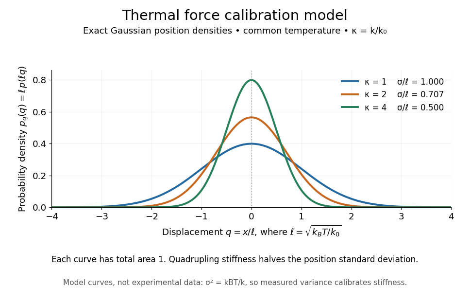
Thermal force calibration model: exact Gaussian position densities for relative trap stiffnesses 1, 2 and 4 at a common temperature
. Details. 
Here , and . The plotted density per unit is . Each curve has total area one; their dimensionless standard deviations are , and . The curves are exact model densities, not noisy experimental data.
Brownian motion becomes a measuring tool: a calibrated position measurement supplies , and the known temperature supplies . Once is known, a slowly applied constant external force shifts the mean by , so in the same harmonic range. Fluctuations therefore calibrate the conversion from displacement to force. Svoboda and Block used this equipartition theorem method when calibrating their bead traps. [ref]
https://www.andrew.cmu.edu/course/42-620/handouts/svoboda_cell_94.pdf. Svoboda and Block, 1994, trap stiffness calibration
.For the example stiffness and , and . Using a variance measured in uncalibrated detector units would not determine that physical stiffness. Measurement noise, finite exposure time, drift and insufficient sampling of the correlated Brownian motion can bias the estimate; record positions over many optical trap relaxation times and account for the detector response. The deterministic relaxation curve above describes relaxation without thermal forcing; an individual thermal trajectory continues to fluctuate.
Optical trap relaxation time 2026-10-14
For a bead in a stationary viscous liquid, linear drag often dominates inertia on the observed timescale. Neglecting both inertia and the random thermal force, the deterministic force balance givesHere is the drag coefficient and the optical trap relaxation time: the time to reduce the deterministic displacement by a factor . The bead approaches equilibrium without oscillation in this overdamped model. The approximation requires times long compared with the inertial time and, for separated timescales, , where is the bead's mass. For a no-slip spherical bead of radius in an unbounded liquid of dynamic viscosity , Stokes drag law gives . Nearby walls change that drag coefficient.
For example, , and give and . A displacement of gives a restoring force of magnitude , and its deterministic displacement drops to after one optical trap relaxation time. These are predictions for the stated model, not measured trajectories.
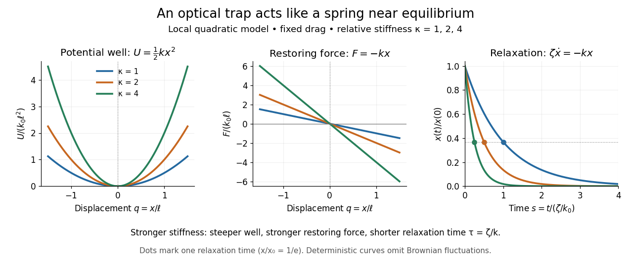
Local harmonic optical trap: potential well, restoring force and deterministic overdamped relaxation
. Details. 
The figure uses , and , with arbitrary positive reference length and stiffness . Thus , and, from , . At fixed drag, greater stiffness gives both a steeper potential energy well and faster relaxation. Thermal Brownian motion is omitted from these deterministic curves.
Poisson integral on the unit disk 2026-10-14
The disk Poisson integral is the harmonic function with boundary data , given byIt is the real part of the Schwarz integral on the unit disk for real data. The nonnegative kernel has integral one; smooth boundary data extend smoothly to the circle. This disk formula should be distinguished from the half-plane formula.
A locally uniformly bounded sequence of harmonic functions with a pointwise limit converges uniformly on compact subsets, and its limit is harmonic. A radial mollifier of fixed local radius reproduces each harmonic function by the mean value property for harmonic functions. Differentiating that convolution gives uniform interior gradient bounds, hence equicontinuity. A finite covering of a compact set converts pointwise convergence to uniform convergence. Passing to the limit in the radial convolution identity proves smoothness; passing to the limit against the Laplacian of each test function proves harmonicity.
Pluriharmonic function 2026-10-14
A smooth real function on a complex manifold is pluriharmonic if . A complex-valued function satisfies the same equation exactly when both real and imaginary parts are pluriharmonic. Restrictions to complex coordinate lines are harmonic functions. On a compact connected complex manifold, choose a maximum of and apply the harmonic maximum principle successively along coordinate lines; the function is constant on a polydisc, then on the manifold by open-and-closed propagation. Without connectedness, constancy is componentwise.
Harmonic functions of Brownian motion 2026-10-14
For a harmonic function and Brownian motion stopped before leaving its domain, Itô formula gives . The drift vanishes. On a compact subdomain, the stopped process is a bounded martingale. Optional stopping theorem at an almost-surely finite exit time therefore gives the boundary mean formula. At the centre of a disk, rotational invariance of planar Brownian motion makes the exit law uniform on the boundary circle. This proves the mean value property for harmonic functions probabilistically.
Kelvin transform 2026-10-14
In three-dimensional Euclidean space, spherical inversion together with the displayed weight maps harmonic functions to harmonic functions on the inverted domain. The Laplacian satisfies . The formula is for ; a new singularity may occur at the origin.
Gradient of a dipole potential 2026-10-14
Harmonic Hardy space of the upper half-space 2026-10-14
For the upper half-space , this is the space of harmonic functions with finite norm . It differs from an analytic Hardy space: no holomorphic function condition is imposed, and its boundary object can be a singular finite Borel measure.
Harmonic odd reflection across a hyperplane 2026-10-14
A harmonic function on one side of a hyperplane that is continuous up to an open portion of the hyperplane and zero there extends harmonically by odd reflection. One local proof takes a ball centered on the boundary and assigns odd continuous boundary data on its sphere. The Poisson integral on the ball is odd, so it vanishes on the equatorial disk. Uniqueness by the maximum principle for harmonic functions identifies it with the original function on the half-ball. Thus the odd extension is harmonic near each boundary point. A globally bounded zero-boundary harmonic function on a half-space is consequently zero by the Liouville theorem for harmonic functions.
Componentwise harmonic vector field Created 2026-10-14 Updated 2026-10-18
A vector field in Euclidean space is componentwise harmonic when each Cartesian component is a harmonic function, equivalently its componentwise Laplacian vanishes. Constant and linear vector fields are examples, as are constant linear combinations of derivatives of away from the origin in three dimensions. Such fields supply the vector potentials in the Papkovich–Neuber representation. Componentwise harmonicity does not by itself require zero divergence or zero curl.
F. and M. Riesz theorem 2026-10-14
If a finite complex Borel measure on the circle has Fourier coefficients for all , then it is absolutely continuous with respect to arc length. The reflected Fourier convention gives the equivalent theorem with positive coefficients vanishing. The Poisson integral on the unit disk is analytic because of the one-sided Fourier spectrum. Subharmonic comparison for its square root and an maximal estimate produce an integrable radial maximum. This maximum dominates the weak-star boundary measure, forcing absolute continuity of measures. The same proof on the real line says that a finite measure with Fourier transform of a finite measure supported in has a Lebesgue density.
H-infinity space 2026-10-14
This Hardy space consists of bounded holomorphic functions on the unit disc, with norm . Its almost-everywhere boundary realization follows from the Fatou theorem for bounded holomorphic functions.
H1 space on the unit disk 2026-10-14
This Hardy space consists of holomorphic functions with , where is normalized angular measure. The H1 non-tangential maximal inequality on the disk controls their approach to the boundary, and the Carleson embedding theorem on the disk characterizes measures against which all these functions remain integrable.
Major arc 2026-10-14
In a circle-method problem of scale , major arcs are neighborhoods of reduced rational points with small denominator, where the relevant exponential sum is approximated using distribution in residue classes. For the three-prime problem one may take and , with suitably fixed .
Minor arc 2026-10-14
Singular series Created 2026-10-14 Updated 2026-11-05
A singular series assembles the local congruence densities in an additive counting asymptotic. For three prime summands it is , with Ramanujan sum . Its Euler product vanishes for even and has a uniform positive lower bound for odd . Different additive problems have different local factors, so this is a specific instance rather than a universal formula.
There are unlisted articles, also show them or only show them.