
Joint entropy Created 2026-10-14 Updated 2026-10-25
Joint entropy is the information entropy of an entire random vector, treating its coordinates together as one outcome. For random variables with finite alphabets and joint probability mass function ,It is measured in bits. The distinction from separate information entropies is whether shared uncertainty is counted once or repeatedly. Two copies of the same fair bit have joint entropy one bit, since only and can occur. Two independent fair bits have joint entropy two bits, since all four pairs are possible and equiprobable.
For a less symmetric example, assign probabilities to respectively. ThenHere is fair, while . Thus and bits, where is binary entropy. Adding the separate information entropies would give approximately bits, overcounting by the mutual information bits.
The chain rule for information entropy makes the shared information explicit:In this example is certain given and fair given , so its average conditional entropy is bit. Sending the first coordinate changes how much uncertainty remains in the second. A prefix code with codewords
0, 10, 11 for the three possible pairs has average length bits, exactly the joint entropy in this stipulated law.For finite alphabets,The lower bound follows because knowing the full random vector determines every coordinate; the upper bound follows from conditioning reduces entropy in the chain rule for information entropy. Equality in the upper bound means joint independence. The difference from that upper bound is total correlation, whose noisy parity total correlation example shows why separate pairwise comparisons need not find all the dependence.
Vacuum domination by a scalar field 2026-10-14
A homogeneous canonical scalar field with positive scalar potential has energy density and pressure . When its potential energy dominates its kinetic energy, the equation-of-state parameter approaches . If other components and spatial curvature are negligible, the Friedmann acceleration equation gives accelerating expansion. Small initial kinetic energy is not enough to ensure long cosmic inflation; the field must also remain on a sufficiently flat part of the scalar potential, as measured by the potential slow-roll parameters.
Inflaton potential 2026-10-14
The inflaton potential is the potential energy density of an inflaton as a function of its field value. Its derivative enters the inflaton equation of motion, while its slope and curvature enter the potential slow-roll parameters.
Fourth-power sum cannot be a square 2026-10-14
Choose a primitive counterexample with minimal and even. Its Pythagorean triple has , . Modulo four forces odd and even, so and . The primitive triangle then has a parametrization with and . Coprimality makes , giving with . This contradicts infinite descent.
Essential infimum and essential supremum Created 2026-10-14 Updated 2026-10-25
The essential infimum and essential supremum describe the lower and upper bounds of a measurable function after disregarding null sets for a specified measure. A pointwise infimum or supremum sees every input; an essential bound sees whether values below or above a proposed threshold occur on a set of positive measure. Thus "essential" means insensitive to changes on a null set, rather than insensitive to unusual values. This distinction makes essential bounds compatible with Lebesgue integrals and the equivalence classes used in Lp spaces. [ref]
Lp spaces (Chapter 7 of Measure Theory). Hunter, Measure Theory, Definitions 7.1, 7.3–7.4: almost-everywhere equivalence and essential bounds
.For a real measurable function on a measure space , the definitions areThese can take values in the extended real number line. On a space of positive total measure, finite essential bounds obey almost everywhere. If is finite, every threshold has ; the corresponding lower-edge statement is for every . These are the measure-based counterparts of the approximation property of a supremum and approximation property of an infimum.
Here is a two-sided example on with Lebesgue measure:The pointwise bounds are and , while the essential bounds are and . Both exceptional singletons are null sets. But for , the inputs where still have measure , and those where have measure : deleting or adding two individual inputs cannot change those lengths. Hence neither essential bound can be moved inward.
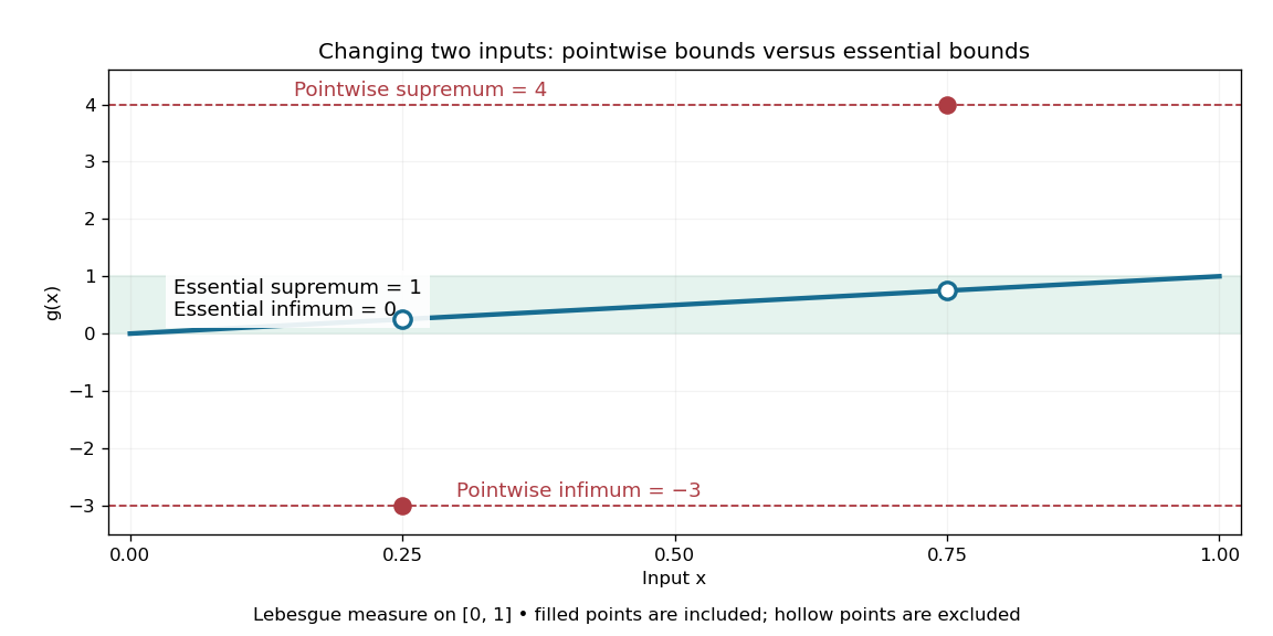
Essential infimum and essential supremum ignore two exceptional singletons, while pointwise infimum and supremum retain them
. The function follows except for the filled values and . Hollow markers exclude the ordinary values at those inputs. The shaded horizontal band spans the essential bounds zero and one for Lebesgue measure. Details.
The choice of measure is part of the answer. The same has essential bounds and under counting measure, because every nonempty set has positive measure. Under the Dirac measure at , both essential bounds equal . A null set for one measure need not be a null set for another.
Nor must the exceptional inputs be isolated. The Dirichlet function, equal to one at rational numbers and zero at irrational numbers, has pointwise supremum one on , but essential supremum zero for Lebesgue measure: the rational numbers form a countable set that is a null set, even though they are dense. Conversely, a value ten on an interval of length affects the essential supremum just as decisively as it would on half the domain. Small positive measure is not zero measure.
Induced character 2026-10-14
For a character of , the induced character isThis is the character of a representation of . Substituting this expression into the character inner product and putting proves Frobenius reciprocity.
Every complex irreducible representation of a finite p-group is induced from a one-dimensional representation of a subgroup. Induct on the group order. Nonfaithful representations reduce to a smaller quotient. For a faithful representation of a nonabelian group, choose an abelian normal subgroup not contained in the centre. Restriction cannot be isotypic, since it would make that subgroup scalar and faithfulness would then force it central. The Clifford correspondence induces the representation from a proper subgroup; induction there and transitivity of induction complete the proof. Abelian groups have only one-dimensional complex irreducible representations.
Unnormalized parabolic induction Created 2026-10-14 Updated 2026-11-05
For a smooth linear character of a parabolic subgroup , unnormalized induction consists of smooth functions satisfying , with right-translation action. The quotient is compact for the local general linear groups in question. Normalized induction inserts a square root of the parabolic modulus in the covariance, changing formulas for the inducing linear character.
Extension of a faithful representation from an open normal subgroup Created 2026-10-14 Updated 2026-10-25
Let be an open normal subgroup of a compact topological group , and let be a continuous faithful representation. Choose representatives for the finite left cosets . Write and act on the -th summand of by into the -th summand. The cocycle identity proves this is a continuous group representation. An element outside has a nontrivial coset permutation, while an element of acting trivially has on the identity-coset summand. Hence the representation of is faithful and integral.
Rice's theorem 2026-10-14
Every nontrivial extensional property of partial computable functions or computably enumerable languages is undecidable.
Degree-ordered independent-set entropy bound 2026-10-14
Order vertices by nonincreasing positive degrees , and let count preceding neighbors. The Madiman-Tetali inequality applied to preceding-neighbor sets and copies of singleton bounds the entropy of a uniformly chosen independent set. In each local term, all-zero neighbor assignment permits two choices at , while every other assignment permits at most one. The maximum-entropy bound gives for that term. Complete bipartite graphs attain equality when one part is ordered before the other.
Independent transversal Created 2026-10-14 Updated 2026-10-20
For a graph whose vertices are partitioned into parts, an independent transversal is an independent set containing exactly one vertex from each part. If a cycle's parts each have twelve vertices, choose one vertex uniformly and independently per part. A cycle edge joining distinct parts is selected at both ends with probability . Each event depends on at most others, since each part meets at most cycle edges. The Lovász local lemma applies because , proving existence for an arbitrary such partition.
Fichtenholz-Kantorovich independent family 2026-10-14
For every infinite set there is an independent family of sets consisting of subsets of . One construction uses a set of pairs , where is finite and . For each , let . Given distinct , choose a finite distinguishing all their traces and choose to contain precisely the traces prescribed to have value one. This realizes every finite Boolean choice. With the axiom of choice, , so a bijection transports this family to . Its independent assignments give distinct ultrafilters.
Expand every term in finitely many generators as a finite nonempty sum of monomials, and associate its exponent support with the upward-closed subset of that it generates. The reverse-inclusion well-quasi-ordering of monomial ideals supplies an earlier support upset containing a later one. Every later monomial is then a multiple of an earlier monomial, hence is absorbed by it under . The earlier sum absorbs the later sum. Thus every infinite term sequence has an earlier element preceding a later one in the reverse natural order. Reflexivity, antisymmetry and transitivity follow directly from commutative idempotent addition.
First-cousin inbreeding coefficient Created 2026-10-14 Updated 2026-11-05
For an otherwise outbred pedigree, each of the two shared grandparents contributes to the kinship coefficient of first cousins. Thus their child has inbreeding coefficient . Equivalently, cousin kinship is one quarter of the kinship of their sibling parents.
// Target: biology.bigb
Inbreeding genotype frequencies Created 2026-10-14 Updated 2026-11-05
For a biallelic locus with frequencies and , and inbreeding coefficient , ancestral-copy identity with probability gives genotype probabilities , and . In the IBD component both copies equal a single ancestral draw; in the remaining component the two ancestral alleles are independent biological population draws. A fully penetrant recessive disease therefore has risk .
// Target: biology.bigb
Importance sampling of a Cauchy tail Created 2026-10-14 Updated 2026-10-25
For uniform on , has density on . The importance sampling weight for the standard Cauchy distribution tail is , and its expectation is the target tail probability. Writing gives and by integrating . The weight varies only between and , making its variance much smaller than that of a rare-event indicator. This is a comparison of sampling variances, not a deterministic ordering of every pair of empirical variance estimates.
Preimage 2026-10-14
For a function and a subset , its preimage isIt is a subset of the original domain of a function. The notation does not require an inverse function: the preimage of a singleton set can have no members, one member, or many members. In the finite example, , and . The preimage of a singleton set is also its fiber of a function.
For subsets , preimages preserve both unions and intersections:For the intersection, the same input belongs precisely when its single output belongs to both and . There is no opportunity to choose different witnesses, which is what made the image counterexample fail. The identities also hold for arbitrary families of output subsets.
In the finite example, choose and . ThenThe intersection of the two preimages is exactly the same set . Complements are preserved with respect to the appropriate source and target sets:For example, the unused output three contributes no extra input: with , both sides of the complement identity are . See Lebl, Proposition 0.3.15: preimages of unions, intersections and complements.
This makes preimages useful for transporting conditions. The solution set of is , and a zero set is a preimage of zero. Requiring two output conditions takes the intersection of their preimages. In topology, a continuous function pulls every open set back to an open set; a measurable function pulls the specified measurable sets in its codomain back to measurable sets in its domain of a function. These definitions use preimages because their set operations remain consistent even when the function is noninjective.
Lux Created 2026-10-14 Updated 2026-11-05
The lux is the unit of illuminance: one lumen of luminous flux uniformly incident on one square metre gives one lux. It measures illumination arriving at a surface, rather than the surface's luminance or the source's luminous intensity.
For a small source of luminous intensity , normal incidence at distance gives when the source can be treated as a point and intervening losses are negligible. Thus a source gives at and at . A meter's sensor must be oriented consistently because tilting changes the projected collecting area.
Mayer's relation 2026-10-14
Mayer's relation states that the difference between heat capacity at constant pressure and heat capacity at constant volume for a fixed-composition ideal gas isHere both capacities are total heat capacities in , is amount of substance, is the number of particles, is the molar gas constant and is the Boltzmann constant. In other normalizations the same statement isThe first is a difference of molar heat capacities, in ; the second uses specific heat capacities, in . Writing with total capacities would omit the sample's amount of substance. The relation holds pointwise even when the capacities depend on temperature. [ref]
https://openstax.org/books/university-physics-volume-2/pages/3-5-heat-capacities-of-an-ideal-gas. Samuel J. Ling, William Moebs and Jeff Sanny, University Physics Volume 2, §3.5: ideal-gas capacity difference
The proof outline is short: enthalpy is , and internal energy of an ideal gas is independent of volume at fixed temperature. Differentiating at fixed composition and amount of substance therefore gives . It uses the ideal gas law, rather than assuming any particular number of molecular degrees of freedom. At fixed pressure, the additional heat supplies expansion work, . The two processes can have the same temperature endpoints and equal while requiring different heat inputs.
For one mole of the rigid-rotation diatomic ideal gas model, and . Heating by with gives in a rigid sealed vessel and under a frictionless piston at fixed pressure. Both gain of internal energy, while the piston delivers approximately of work. This is a calculated model budget. If the capacities vary with temperature, the corresponding finite statement is stillunder the fixed-pressure and fixed-volume heating assumptions in heat capacity. Their final volume values generally differ. Combining Mayer's relation with heat capacity ratio also gives and locally; constant values cannot be extrapolated across intervals in which changes.
For a smooth stable single thermodynamic phase of a general simple compressible system, the broader Maxwell relation identity iswhere is the coefficient of thermal expansion and the isothermal compressibility, with composition fixed throughout. Substituting the ideal gas law gives ; a real gas need not do so. This distinction matters near a phase transition or when interactions appreciably change the equation of state. It explains why Mayer's relation is useful: thermal measurements under different constraints become linked to a mechanical response, while the difference retains a particularly simple value for an ideal gas.[ref]
There are unlisted articles, also show them or only show them.