
A test cross crosses an individual with a homozygote for recessive alleles, allowing suitable offspring phenotypes to reveal transmitted gamete combinations.
Independent assortment means that transmission at different genetic loci has conditional independence given the parental genotype. With fair Mendelian segregation, a parent heterozygous at two genetic loci, , produces gametes with probability each. For example,Here labels an allele combination; it does not assert that the two genetic loci lie on the same chromosome.
The physical model is stochastic orientation of different homologous chromosome pairs toward the two poles of the spindle apparatus in meiosis I. One pair's orientation does not determine another's. For two pairs, one division can send together and together; another can send together and together. See The Process of Meiosis (§11.1, Metaphase I and Figure 11.5: random orientation of chromosome pairs).
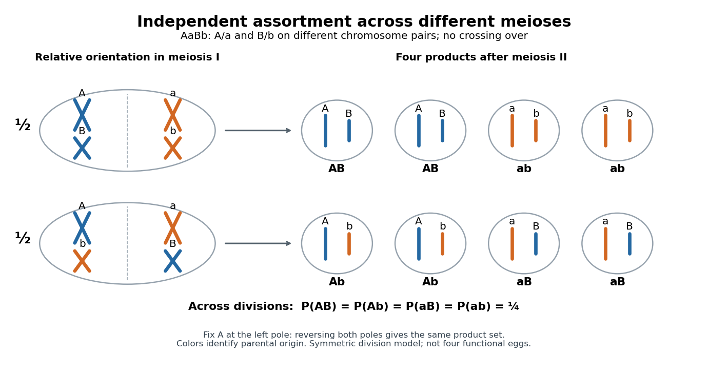

With distinguishable homologous chromosome pairs, there are choices of parental homologous chromosome origin for a product at a specified pole, each with probability under this model. For , enumerate , where M and P mark parental origins. Whole-pole reversal pairs complementary choices, leaving unordered partitions for . For there are four choices for a specified pole but only the two relative orientations drawn. This counts possible products across meioses, not eight different products of one division when . Identical alleles at scored genetic loci can also make different parental-origin choices observationally indistinguishable.
Independent assortment of different chromosome pairs does not imply independence of every pair of genes. Nearby genetic loci on the same chromosome can show genetic linkage. Chromosomal crossover can create new haplotypes, but does not automatically erase genetic linkage. See Laws of Inheritance (§12.3, Law of Independent Assortment and Linked Genes Violate the Law of Independent Assortment). In the ordinary fair two-locus model with parental haplotypes and recombination fraction ,Thus gives only the two parental haplotypes, while gives four equal probabilities. A recombination fraction of alone does not establish that the genetic loci lie on different chromosomes.
A motivating experiment appears in Experiments in Plant Hybridization by Gregor Mendel (§9, “The Reproductive Cells of the Hybrids”). In peas, hybrids for round versus wrinkled seeds and yellow versus green seeds were crossed reciprocally with constant wrinkled-green plants. The readout was visible seed shape and color: hybrid seed parents gave 31 round-yellow, 26 round-green, 27 wrinkled-yellow and 26 wrinkled-green; the reciprocal cross gave 24, 25, 22 and 27.
The apparatus was controlled pollination: opening immature flowers, removing stamens with forceps, and applying selected pollen to the stigma. Two-year trials established constant parental characters; greenhouse pots checked interference from insects in outdoor beds. Reciprocal crosses tested both transmission directions. These procedures are described in Experiments in Plant Hybridization by Gregor Mendel (§§2–3).
With complete dominance at both genetic loci, this test cross makes each phenotype report one hybrid gamete combination. The ideal expected values are and per class. The observations support four transmitted combinations, approximately equally frequent. They do not directly image chromosome orientation or prove independence for all genes; failed development and seed germination also limit the inference, as §9 notes.
An ordered sequence of memory references, recording repetitions as well as addresses. The example under memory cache records twelve reads in decimal physical addresses; the trace itself does not determine cache hits until cache line size, capacity, initial contents, placement and replacement are specified.
For a terminating pure function, a reusable entry must record its correct completed result, and equal memoization keys must imply equal results throughout the entry's memoization cache lifetime. Reusing that result must also preserve the behavior callers require. These conditions separate correctness from speed: a complete key can be correct even if it rarely repeats.
A procedure using deterministic computation can still have a required side effect. If a procedure returns and appends an audit record on every call, serving the second call from a table preserves the numerical answer but skips the second record. Likewise, if each call promises a fresh mutable list, returning the same stored mutable list changes observable sharing and allows a caller to damage later answers. Plain result reuse is unsuitable for those contracts.[ref]
functools — Higher-order functions and operations on callable objects (Python 3.14 documentation). Python documentation, functools.lru_cache: paragraph warning against functions with side effects, distinct mutable results, or impure time/random results
Completion matters for recursion. Suppose computing key needs key , and computing needs . A table containing only completed answers has no answer to return for the second ; remembering completed values does not make this directed cycle terminate. Marking a key
ACTIVE before descending detects re-entry, as in spreadsheet dependency evaluation, but detection is not a solution of the circular equations. If computation fails, clear its active mark and do not publish an unfinished value. The example using Fibonacci numbers avoids this issue through a strictly decreasing argument.The call counts above assume sequential execution and no eviction. Concurrent requests for an absent key can both begin evaluation before either publishes its result; keeping a table coherent alone does not ensure one body execution per key.[ref]
functools — Higher-order functions and operations on callable objects (Python 3.14 documentation). Python documentation, functools.cache and functools.lru_cache: thread-safe cache updates can still allow repeated evaluation before completion
Under constant-cost lookup and integer addition, Memoized Fibonacci evaluation has time complexity in Big O notation, retaining values. A hash table needs its own lookup-cost assumptions; an array indexed by avoids hash collisions in this example. Memoization removes repeated bodies, but also pays for keys, lookups and retained answers. A workload without reuse can pay those costs without saving evaluations.
The call stack remains. Left-first recursion descends through arguments before returning, giving simultaneously active frames for . Therefore the auxiliary space complexity includes frames as well as table entries in the constant-size-value model. An iterative bottom-up dynamic programming calculation removes these recursive frames; retaining only the two previous Fibonacci numbers suffices when only the final value is wanted, but discards the table useful for later requests.
Exact Fibonacci numbers do not remain constant-size values. For , the recurrence relation gives , so the representation of as a binary number has order bits. With ordinary addition costing order bit operations on such operands, the additions cost order bit operations in total. Retaining all values also requires order bits of value storage, before keys and frame overhead. The linear bound counts additions under its stated cost model; it is not a linear bound on exact integer arithmetic in bits.[ref]
Lecture 15: Recursive Algorithms (6.006 Spring 2020) by Massachusetts Institute of Technology, 6.006 course staff. MIT 6.006 Spring 2020, Lecture 15: Recursive Algorithms, printed p. 3, final three bullets: growing Fibonacci bit lengths and addition cost
The Fibonacci numbers give an exact example. For a nonnegative integer , their recurrence relation isTo obtain by direct recursion, evaluate and separately; computing also evaluates . The full call tree has 15 occurrences but just six distinct arguments, . Shared dependencies form a directed acyclic graph because every directed edge goes to a strictly smaller argument. Memoization evaluates a distinct argument on first demand; filling values in increasing argument order is the corresponding bottom-up dynamic programming calculation.[ref]
Lecture 15: Recursive Algorithms (6.006 Spring 2020) by Massachusetts Institute of Technology, 6.006 course staff. MIT 6.006 Spring 2020, Lecture 15: Recursive Algorithms, printed pp. 2–3, Fibonacci Numbers and Re-using Subproblem Solutions
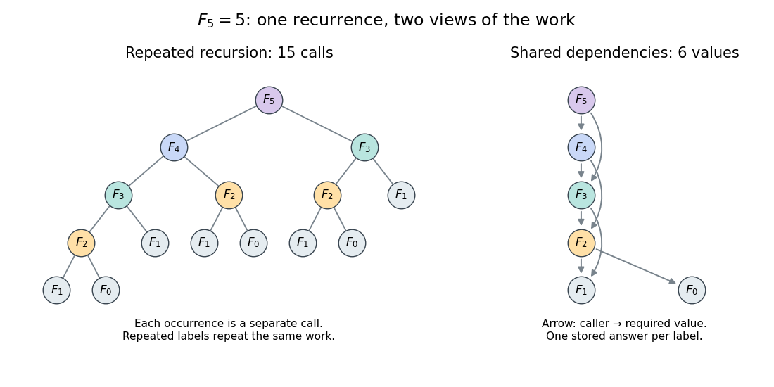
Repeated calls for Fibonacci numbers and their shared directed acyclic graph of dependencies
. The call tree contains 15 occurrences for . The dependency graph contains six distinct arguments and eight directed edges. Equal labels have equal colors; arrows in the right panel point from a caller to the value it requires. Details.
Use an initially empty hash table
memo, shared by every recursive call. Count even the first evaluations of the two base cases, store only completed results, evaluate the left term first, and retain all entries. The following original procedure assumes a nonnegative integer argument:def cached_fib(n, memo):
if n in memo:
return memo[n]
if n < 2:
value = n
else:
value = cached_fib(n - 1, memo) + cached_fib(n - 2, memo)
memo[n] = value
return valueEvery self-call must pass through the memoization lookup. Wrapping only the outer call while leaving inner calls uncached retains the repeated work. Test membership rather than whether the stored value is nonzero: is a valid completed result.
For cold , the lookup arguments are . The first six are absent; the last three reuse completed answers. Results are stored on return in argument order , with values . Thus there are nine wrapper calls, six body evaluations and four additions. Repeating with the same table takes one wrapper call and no body evaluation. Requesting next evaluates only its body, reuses and , and stores : three wrapper calls, one body evaluation and two hits.
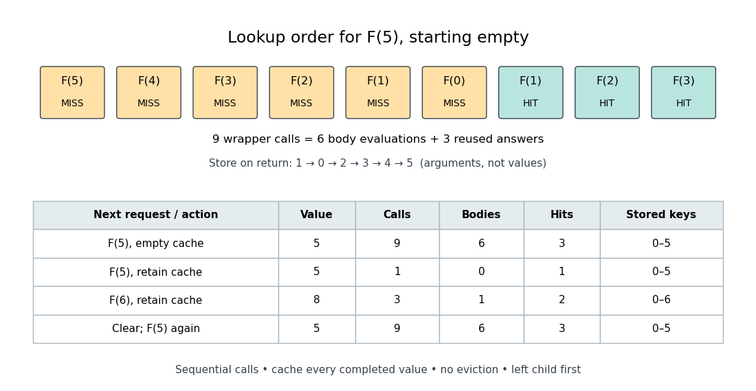
An exact memoization lookup trace and the effect of retaining or clearing its table
. The first row records cold lookup order. The table records successive requests with one retained table; clearing it before the final request restores the cold counts. Calls include lookups that immediately return stored values; bodies count only first evaluations. Details.
The direct-call count satisfies and . Its exact solution is , as substitution into this recurrence relation verifies. With the specified memoization procedure, a cold call at evaluates distinct bodies, makes additions and makes wrapper calls. There are hits: each of the nonbase bodies issues two recursive calls, in addition to the initial call. The difference is between the number of occurrences and the number of distinct subproblems.
Overlapping subproblems occur when several parts of a calculation request the same smaller problem. Memoization can share its answer if the memoization key identifies that problem completely. For the Fibonacci numbers, both and require . In dynamic programming, the dynamic programming state plays the corresponding role of identifying a reusable continuation. Overlap explains potential savings; the recurrence relation and its base cases still need to be correct.
A membrane channel whose opening depends on membrane potential. Regenerative activation and subsequent inactivation or opposing currents help produce an action potential.
A reversal potential is a membrane potential at which a specified open ion channel, or specified combination of ion channels, carries zero net electric current, with the surrounding conditions fixed; the electric current changes sign across that voltage. Specifying which current matters: an individual ion contribution and a sum of several contributions can reverse at different voltages. Zero net electric current does not mean that all ions have stopped moving. See Purves et al., Neuroscience, 2nd edition (2001): reversal of a mixed-ion channel current.
Throughout these examples, membrane potential is , and conventional current is inward-positive. Positive electric current corresponds to net positive electric charge entering or net negative electric charge leaving. Negative electric current corresponds to the reverse charge transfer. A convenient Ohmic approximation iswhere is the available electrical conductance. For fixed , gives positive electric current, gives zero, and gives negative electric current; the line has slope . If , the modeled pathway carries zero electric current at every voltage: closing it does not locate its reversal potential. 3.1 Synapses (§3.1: conductance-based synaptic current) uses outward-positive ; the formula here reverses that sign to match this wiki's inward-positive convention.
For the stipulated single-pathway example from ion channel, and giveThe open ion channel carries zero net electric current at even though remains positive. Near that point a change of membrane potential changes the electric current, which is why zero current at one voltage does not make an open pathway electrically irrelevant; see shunting inhibition.
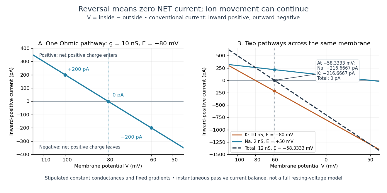
Inward-positive electric current: one reversal and two-channel cancellation
. Original computed curves for stipulated constant electrical conductances and fixed reversal potentials. Left: , . Right: a potassium pathway with , and a sodium pathway with , . Their net electric current vanishes at while both individual electric currents remain nonzero. These are model values, not empirical measurements. Details.
For an ion channel passing only one ion species by passive transport, its reversal potential can equal that species' Nernst equilibrium potential, where the chemical and electrical contributions to electrochemical potential balance. At that thermodynamic equilibrium, passage in both directions can continue with no net transport. For an ion channel admitting several ion species, opposing contributions can cancel while each species continues to have net transport. Such a reversal potential is not generally any one species' Nernst equilibrium potential. See the Purves reference above.
To work out that cancellation explicitly, put two Ohmic ion channel populations across the same cell membrane. Stipulate constant electrical conductances and fixed reversal potentials:The potassium and sodium contributions add because both pathways experience the same membrane potential:Thus . This weighted mean follows simply by expanding and regrouping the two current terms; it assumes additive Ohmic contributions and a positive total electrical conductance. At , the inward-positive individual electric currents areThe potassium contribution is outward and the sodium contribution inward. Equal and opposite electric currents give ; neither pathway has stopped transporting its ions. The calculation treats two distinct pathways. Applying it to one mixed-species ion channel would additionally require a justified decomposition into independent Ohmic contributions; a general mixed-channel reversal potential cannot be obtained by assuming those hypotheses silently.
This is an instantaneous balance of the specified passive electric currents. It would be the stationary voltage of a passive capacitance model containing only these constant pathways and no applied electric current, but it is not a complete prediction of a living cell's resting membrane potential. Other electric currents, voltage-dependent gating, and pumps involved in active transport can matter. Pumps that transfer net electric charge are electrogenic and contribute their own electric current. See Purves et al.: functional properties of the sodium/potassium pump.
The toy model holds ion concentrations and therefore the stipulated reversal potentials fixed. Continuing inward sodium and outward potassium transport would change finite reservoirs unless active transport or external control maintained them. Transport can be a small fraction of the reservoir's ions over a short interval, making fixed concentrations a useful approximation; it is not a claim that the reservoirs never change. See Gerstner et al., Neuronal Dynamics (2014), §2.1: equilibrium potentials, channel currents and maintained gradients.
A reversal potential makes the effect of opening an ion channel predictable from the present membrane potential. The same open pathway can carry inward or outward electric current as crosses its reversal potential. The two-pathway example reveals a particularly useful distinction: zero net charge transfer can coexist with continuing exchange of different substances. That distinction connects membrane transport to electric current measurements without mistaking electrical balance for thermodynamic equilibrium.
Hyperpolarization makes a neuronal membrane potential more negative relative to the exterior. It is a voltage description; inhibition need not produce hyperpolarization, as shunting inhibition illustrates.
For a negative neuronal membrane potential, depolarization raises it toward zero or beyond, making the interior less negative relative to the exterior. This describes a voltage change, not necessarily increased action potential generation; see the depolarizing inhibition example under synaptic potential.
Ploidy counts sets of chromosomes; DNA amount counts material. Let be the number of chromosomes in one complete set and the DNA amount of one unreplicated set. For the ordinary diploid model, read each row per completed cell nucleus, not as a total across all products:
| Stage | Ploidy | DNA amount | Chromosome organization |
|---|---|---|---|
| Before DNA replication | Two unreplicated sets | ||
| After DNA replication | Two sets; each chromosome has two sister chromatids | ||
| After meiosis I | One replicated set | ||
| After meiosis II | One unreplicated set |
In the illustrated example, the starting biological cell has four chromosomes. DNA replication gives eight chromatids, organized into four replicated chromosomes. Each product of meiosis I has two replicated chromosomes, hence four chromatids; each final product has two unreplicated chromosomes. Across completed products, after meiosis I and after meiosis II: division redistributes the replicated DNA. A haploid cell nucleus can therefore have without becoming diploid.
The second division of meiosis separates sister chromatids, without an intervening round of DNA replication.
The first division of meiosis separates replicated homologous chromosomes; their sister chromatids remain associated.
Cited passages: Hunter, Measure Theory, Definition 7.4: the L-infinity norm; Hunter, Measure Theory, Definitions 7.1 and 7.4: Lp spaces and norms; Hunter, Measure Theory, Definitions 7.1, 7.3–7.4: almost-everywhere equivalence and essential bounds; Hunter, Measure Theory, §7.4, Lemma 7.9, pp. 81–82, and Theorem 7.10, pp. 82–83: norm summability and completeness.
There are unlisted articles, also show them or only show them.