Perpendicular fields with and form a null electromagnetic field. The constant-field Lorentz-force generator is nilpotent, so its exponential terminates as a polynomial.
Both invariants of the electromagnetic field tensor vanish for this field class.
Relativistic hyperbolic motion in a uniform electric field by  Codex 0 Created 2026-09-24 Updated 2026-10-14
Codex 0 Created 2026-09-24 Updated 2026-10-14A particle released from rest in a constant electric field parallel to its motion follows a spacetime hyperbola and has rapidity proportional to proper time.
Lorentz boosts mix transverse electric and magnetic field components.
The four-potential combines the electric potential and magnetic vector potential as . The electromagnetic four-potential transforms underwhile the antisymmetric field tensor is unchanged.
Measure theory studies measures, which assign sizes to measurable sets, and the Lebesgue integral, which accumulates values weighted by those sizes. The same framework describes Lebesgue measure on the real numbers, counting measure on discrete collections, and probability measures on possible outcomes. The choice of measure determines what counts as large; the choice of sigma-algebra determines what can be measured.
A striking example separates size from proximity: the rational numbers in form a dense set with Lebesgue measure zero, although the whole interval has Lebesgue measure one. This distinction makes almost everywhere statements useful: exceptional null sets can be ignored in a Lebesgue integral even when they meet every open subinterval. The monotone convergence theorem and dominated convergence theorem then give precise conditions for passing a limit through an integral.
A historical starting point is Lebesgue's 1902 thesis, [ref]
https://www.ime.usp.br/~glaucio/mat5798/textos/aula1.pdf#page=2. Intégrale, Longueur, Aire (original title page reproduced in USP lecture notes)
. Its title connects integration with the geometric task of assigning sizes.A function on a convex set is a convex function if, for every and ,Geometrically, a line segment joining two points of its graph of a function lies on or above that graph of a function. The convex set condition ensures that the intermediate input stays in the domain of a function. An affine function satisfies the defining inequality with equality.
For the quadratic function , the inputs and have equally weighted arithmetic mean . Evaluating at the arithmetic mean gives , whereas averaging the outputs gives . Averaging first saves one unit in this example. More generally, direct expansion givesThis identity proves convexity and also shows exactly when its defining inequality is strict.
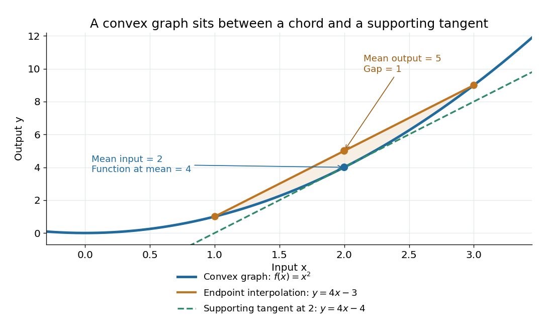
The graph of a convex quadratic lies below its endpoint interpolation and above its supporting tangent
. For , the line segment through and has height at , while the graph of a function has height . The tangent line is an affine minorant: everywhere. Details.
For a differentiable convex function, the tangent line in one dimension, or the corresponding supporting affine function in several dimensions, lies below the entire graph of a function. This is the subgradient inequality. The equivalent geometric statement is that the epigraph, consisting of points on or above the graph of a function, is a convex set. These characterizations are developed in Boyd and Vandenberghe's convex-function slides, sections 3.1–3.4.
Convexity does not require differentiability: the absolute value function is a convex function with a corner at . When a function is twice continuously differentiable on an open interval, it is a convex function exactly when its second derivative is nonnegative throughout that interval. In several dimensions, the corresponding criterion on an open convex set is that its Hessian matrix is positive semidefinite everywhere. The domain of a function matters: is a convex function on , but not on all of . A strictly positive second derivative is sufficient for strict convexity, but is not necessary: is a strictly convex function although its second derivative vanishes at .
The usefulness of convexity is that local information can certify a global conclusion. Every local minimum of a convex function on a convex set is a global minimum: if a lower value existed elsewhere, the defining inequality would produce lower values arbitrarily close to the proposed local minimum. For a differentiable convex function on an open convex set, a zero gradient therefore certifies a global minimum. Strict convexity gives uniqueness when a global minimum exists; it does not supply existence by itself. These facts explain the role of convex functions in convex optimization.
A convergent subsequence of is a sequence with strictly increasing indices that converges to a limit.
For a nonempty set , a real number is its infimum precisely when it is a lower bound and every other lower bound is at most . It is the greatest lower bound, not necessarily the minimum.
For , zero is a lower bound. Every positive candidate fails: the Archimedean property gives an integer , hence . Thus , although zero is never a member of . This is the lower-edge counterpart of approximating an unattained supremum.
For a nonempty set , a real number is its supremum precisely when it is an upper bound and no smaller real number is an upper bound. It is unique: two least upper bounds must each be no greater than the other.
For , every number at least one is an upper bound, and none smaller than one bounds the whole set. Thus , although . For , that same supremum is also the maximum. The approximation property of a supremum supplies witnesses arbitrarily close to an unattained upper edge.
Calculus connects local change with accumulated change. A derivative asks how fast a function changes near one input; an integral adds its contributions across an interval. The fundamental theorem of calculus explains why these operations fit together: accumulating a continuous rate produces a quantity whose derivative is that rate.
For example, suppose a particle moves along a straight line with position metres at time seconds. Its velocity is metres per second. Between and , adding the velocity over time givesHere the velocity stays positive, so the displacement also equals the distance travelled. If the particle reverses direction, the integral of its signed velocity still gives displacement, while the integral of its speed gives total distance.
This is useful because local rules are often easier to specify than whole trajectories. A differential equation can prescribe a particle's velocity or a population's growth rate; integration then reconstructs its evolution, subject to an initial condition. In the other direction, a derivative extracts local information from a known function, and optimization uses that information to locate or approach promising inputs. The same two operations therefore connect measurement, prediction and design.
The visual connection is developed in derivative, integral and fundamental theorem of calculus. The definitions depend on limits, which turn progressively finer finite measurements into exact mathematical statements. A graph with a corner need not have a derivative there, and the conditions permitting integration or interchange of limits matter; calculus is more than a collection of symbolic rules.
Historically, Isaac Newton described changing quantities and their rates in the language of fluents and fluxions; his manuscript History of the Method of Fluxions records that approach.[ref]
https://www.newtonproject.ox.ac.uk/view/texts/normalized/NATP00356. Isaac Newton, History of the Method of Fluxions, Cambridge University Library MS Add. 3968
Gottfried Wilhelm Leibniz's Nova methodus pro maximis et minimis appeared in Acta Eruditorum in October 1684, pp. 467–473; the original article is preserved in the HKUST Library collection.[ref]https://digitalcollections.hkust.edu.hk/Detail/objects/b540295. Gottfried Wilhelm Leibniz, Nova methodus pro maximis et minimis, 1684
The modern limit definitions used here should not be read back into those seventeenth-century formulations.A sequence is an ordered family indexed by the natural numbers; a series studies the partial sums of a sequence of terms.
An Lp norm measures the size of a measurable function by averaging a power of its absolute value with respect to a specified measure. For ,when the integral is finite. The exponent controls how strongly large values influence the result. The Lp space identifies functions equal almost everywhere, so this becomes a norm on the corresponding equivalence classes. For , use the essential supremum of , as defined by the L-infinity norm. [ref]
Lp spaces (Chapter 7 of Measure Theory). Hunter, Measure Theory, Definitions 7.1 and 7.4: Lp spaces and norms
.For a two-coordinate vector , treat the coordinates as a function on two inputs with counting measure. Then , , and . The middle case is the Euclidean norm; the first adds the coordinate magnitudes, and the last takes their largest value. These are different answers to different questions about size, all satisfying the triangle inequality.
If instead each input has probability , the same values give and , while remains unchanged. Thus the measure is not an optional label. On a probability space, the finite Lp norms are nondecreasing in whenever they are finite, by Hölder's inequality; the unnormalized two-coordinate example above decreases instead. Statements comparing different exponents must specify their measure convention.
Why are these sizes useful? If is an error function, its L1 norm measures aggregate absolute error, its L2 norm measures the square root of aggregate quadratic loss, and its L-infinity norm bounds error almost everywhere. Concentrating a large error on a set of small positive measure can give a modest finite Lp norm but a large L-infinity norm. The three-point example and diagram in L-infinity norm show this explicitly, including why a null set behaves differently from a rare event.
A real-valued function on a normed vector space is coercive when its value tends to positive infinity as the norm of its argument tends to infinity. A continuous coercive function on a finite-dimensional real vector space attains a global minimum.
A real-valued function that is continuous on a nonempty compact space attains both a global minimum and a global maximum. In particular, for a continuous function on a nonempty closed interval, there are points such thatThe important word is “attains”: the best values occur at actual allowed inputs, rather than merely being approached. The interval version is [ref].
For a worked example, take on . Its global minimum is , and its global maximum is . Nonnegativity gives the first answer; on the specified closed interval gives the second. The endpoint is essential: looking only for a zero derivative would find the minimum and miss the maximum.
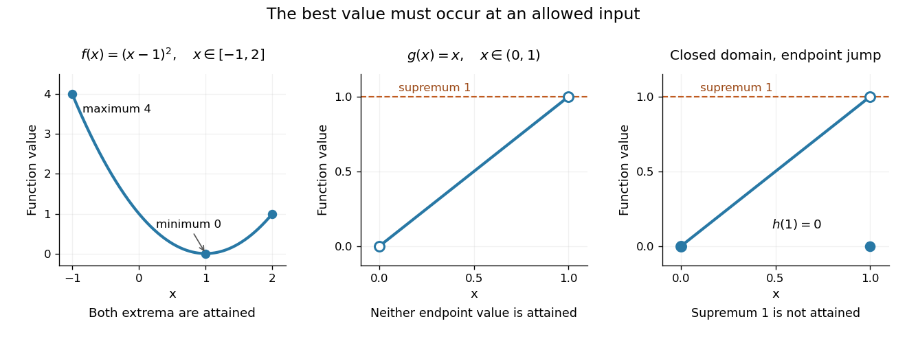
An attained minimum and maximum on a closed interval, compared with excluded endpoints and a discontinuous endpoint value
. Details. 
For comparison, the continuous function on the open interval has infimum and supremum , but neither is a value of . Even a closed domain is insufficient without continuity: define for , and . On , its supremum is , approached by for , but every function value is strictly less than . This endpoint change makes discontinuous, preventing attainment. On the unbounded real line, the continuous function has neither a global minimum nor a global maximum. These examples show what can fail when a hypothesis is dropped; functions outside the hypotheses may still have extrema.
The extreme value theorem is an existence tool for optimization: first establish that a continuous objective function on a nonempty compact feasible set has a best value, then investigate where it occurs. It neither locates the optimizing point nor promises uniqueness or differentiability. For example, the absolute value function on has its global minimum at zero although no derivative exists there; a constant function has every input as a minimizer. This role in optimization is explained in University of Toronto MAT237 notes, section 1.4: compactness and the extreme value theorem.
A short proof outline identifies the mechanism. The continuous image of a compact space is compact; a nonempty compact subset of the real line contains its infimum and supremum. For a closed interval, one can instead choose inputs whose outputs approach the supremum, extract a convergent subsequence by the Bolzano-Weierstrass theorem, and use continuity to make its limiting output equal that supremum. The closed interval retains the limiting input. Repeating the argument for the infimum supplies the minimum.
There are unlisted articles, also show them or only show them.