
Probability inequalities bound event probabilities from limited information, such as moments, without requiring a complete probability distribution. Markov's inequality uses a nonnegative random variable's expected value; Chebyshev's inequality uses a variance to bound deviations from a mean. The attraction is a guarantee that applies to many possible probability distributions. Their bounds can be conservative for a particular model, and distributions attaining equality show when the available information really cannot give more.
An expected value is the probability-weighted arithmetic mean of a real-valued random variable. On a probability space , its general definition is the Lebesgue integralwhere is the probability distribution of . For an integrable random variable, this is a finite real number. With a probability mass function , use ; with a probability density function , use . These are two ways of computing the same weighted average, rather than different definitions for different experiments.
For example, suppose takes the values with probabilities . ThenThe most likely outcome is , and is not a possible outcome at all. The expected value summarizes all outcomes and their weights; it need not predict the result of one trial. Geometrically, placing masses equal to the probability masses at the outcome positions gives a center of mass at , since . This balance-point interpretation also explains the connection to a weighted arithmetic mean. [ref].
For the dimensionless random variable with probability density function on , the expected value is . Integrating the probability density function itself gives one; to compute the expected value, multiply by the outcome first. [ref]
https://ocw.mit.edu/courses/18-05-introduction-to-probability-and-statistics-spring-2022/mit18_05_s22_class06-prep-a.pdf. Orloff and Bloom, expectation for continuous random variables
.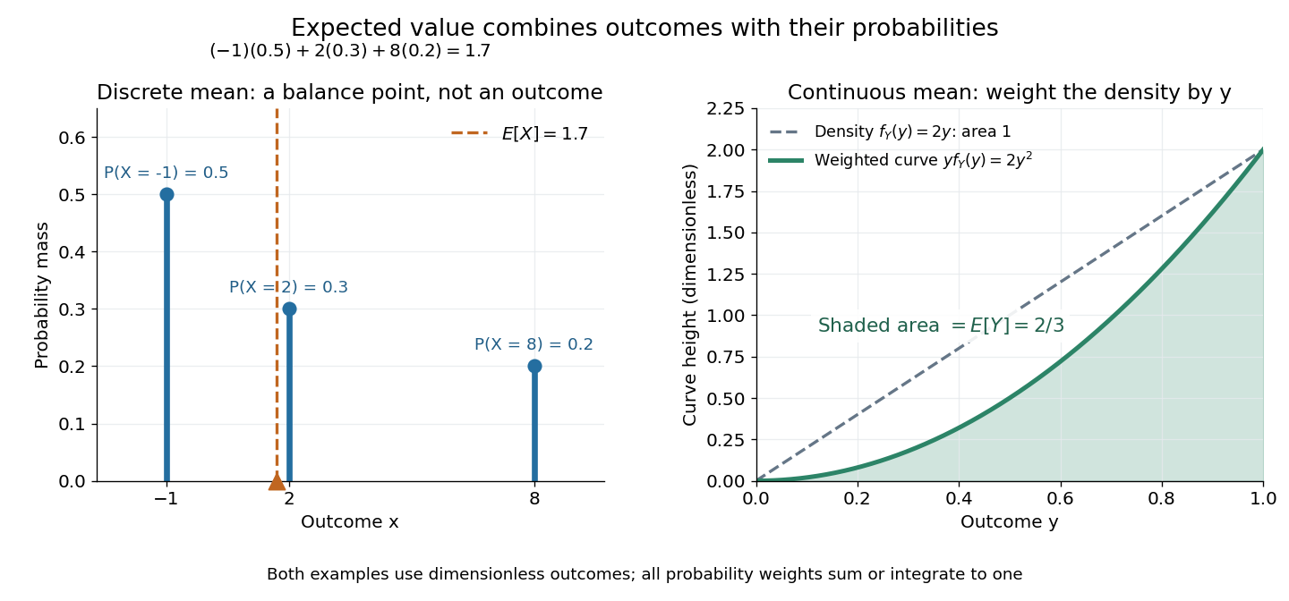
Expected value balances probability masses, or integrates outcomes weighted by a probability density function
. The left panel's dashed line marks , even though the only possible outcomes are . In the right panel, the shaded area under is ; the area under the dashed probability density function is one. Both examples use dimensionless outcomes. Details.Why is this useful? Linearity of expectation lets us compute an average total by adding average contributions, even for dependent random variables. And for independent and identically distributed integrable random variables, the strong law of large numbers says their sample mean approaches their common expected value almost surely. The theorem supplies the link to repeated observations; the weighted-average definition itself does not promise that any particular finite run will be close to the expected value.
There is a useful historical connection to valuing uncertain rewards. In his 1657 De ratiociniis in ludo aleae, Christiaan Huygens assigns the value to equally likely rewards , and when they have equally likely chances. These are the finite weighted-average formulas for expected value. His opening discussion asks how to divide the stakes when a game stops before completion, connecting probability to a concrete question about an unfinished contest. [ref]
https://math.dartmouth.edu/~doyle/docs/huygens/huygens.pdf. Huygens, De ratiociniis in ludo aleae, 1657; reprint of the 1714 English translation, introduction and Propositions I–III
.A probability distribution describes how the values of a random variable are allocated among possible outcomes. More precisely, the law of a random variable assigns each measurable set the probabilityIt is a probability measure on the values of . The underlying experiment can be more elaborate than the output: different experiments may produce the same probability distribution. The law of a random variable retains the probabilities needed to answer questions about that output. [ref]
https://ocw.mit.edu/courses/6-436j-fundamentals-of-probability-fall-2018/9797310bed4c7f5b5d40d007783eec8d_MIT6_436JF18_lec04.pdf. MIT Fundamentals of Probability, Lecture 4: random variables and their laws
.For a finite example, let take values with probability mass function , , . Its probabilities sum to one. The event has probability , whereas has probability : including one endpoint matters when it carries positive probability.
For a contrasting random variable , choose the probability density function on , and zero elsewhere. It integrates to one. Now , while every single outcome has probability zero. The probability density function can have height : probabilities come from integrals over outcome ranges.
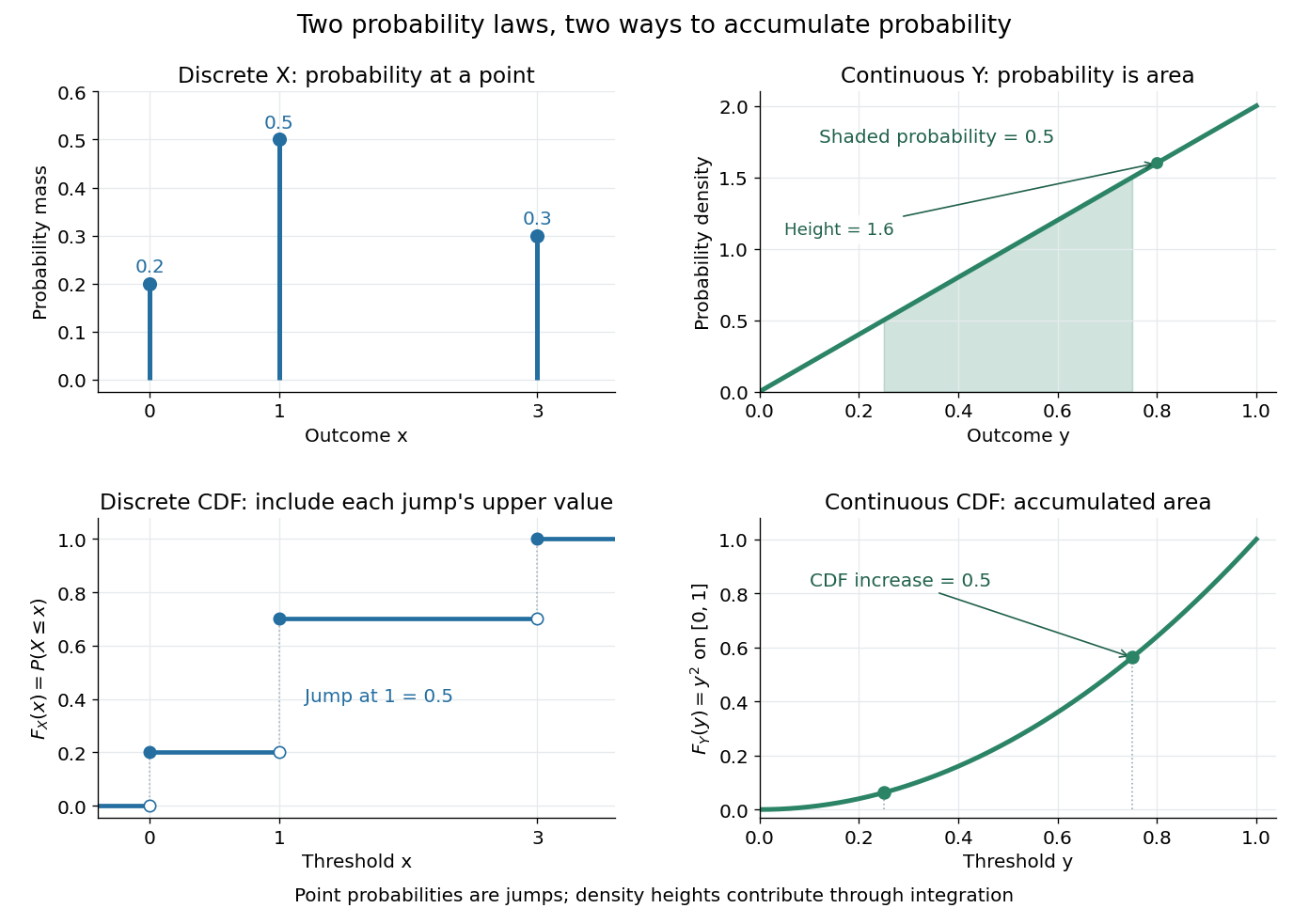
The cumulative distribution function answers all threshold questions for a real random variable, regardless of whether there are jumps or a probability density function. A quantile function reverses the direction of the question: given a cumulative probability level, find a threshold. This connects descriptive summaries to inverse transform sampling, which constructs a chosen probability distribution from a uniform distribution.
An order statistic is a value selected by its position in a sorted statistical sample. For real observations , writeThe th order statistic is the th smallest value, counting repeated values separately. The parentheses distinguish sorted position from the original observation label: and need not be equal. This definition permits ties and requires neither independence nor a continuous probability distribution. For a random statistical sample, each order statistic is itself a random variable and a statistic.
For example, the five fixed observationssort toTheir original indices in sorted order are , so . Their ranks of observations, listed in original observation order, are . Here is the minimum, is the sample maximum, and is the sample median. These are deliberately chosen observations, rather than simulated draws.
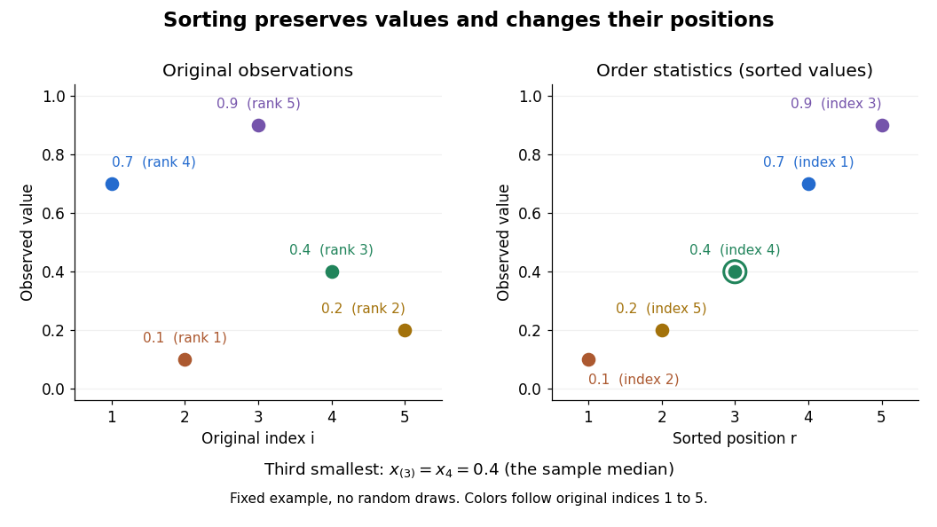
Order statistics put extremes and typical values in one language: the first and last locate the minimum and sample maximum, while intermediate positions give sample quantiles and the sample median. Under the existing generalized-inverse convention, the sample quantile at level is . For the five observations, the sample quantiles at are . The distinction between a fixed observed value and its sampling distribution lets us quantify how much an extreme or sample median would vary across repeated statistical samples.
The useful counting identity isFor independent and identically distributed random variables with a continuous cumulative distribution function , the count on the right has binomial distribution with parameters , givingThis cumulative distribution function is a binomial distribution tail: a question about sorting becomes a question about counting successes in Bernoulli trials. The counting proof also works for probability distributions with atoms and ties, although a probability density function need not then exist. For a uniform order statistic, on , which makes the formula particularly explicit.
A Poisson point process has independent counts on disjoint sets and Poisson count in each set with mean given by its intensity measure.
A Homogeneous Poisson process models arrivals at a constant rate . Its counting process counts arrivals in , with . Its paths are right-continuous nondecreasing functions, take nonnegative integer values, and have unit jumps almost surely. The defining Poisson distribution of each increment isIt has stationary increments: the probability distribution above depends on the duration , not the starting time . It also has independent increments: counts in any finite collection of disjoint time intervals are independent random variables. Together these conditions specify the joint count laws, not merely the Poisson distribution at a single time.[ref]
Poisson Processes (Chapter 2). pp. 78-79: counting-process definition and its equivalence to exponential interarrival times
The rate has units of arrivals per unit time; is dimensionless. The Poisson distribution givesFor a toy rate per minute and a duration of minutes, the expected value and variance of the count are both . The probability of no arrival is , and the probability of exactly three is . In two consecutive one-minute intervals, the probability of exactly two arrivals in the first and exactly one in the second is , using independent increments. These are exact model calculations with rounded decimals, not measured frequencies.
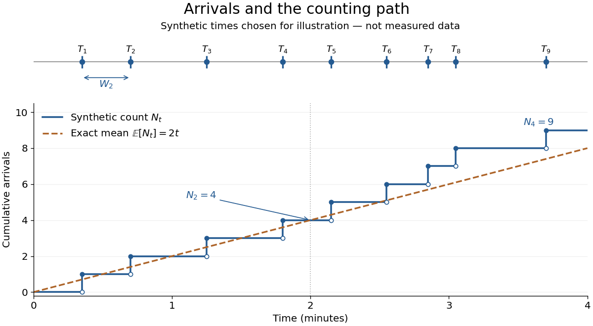
Synthetic arrival times and their right-continuous counting path, compared with the exact mean at two arrivals per minute
. Details. The diagram's nine hand-chosen arrivals illustrate a path; the line is an expected value, not a prescribed trajectory. Constant rate does not imply evenly spaced arrivals. Poisson interarrival times connect the count description to waiting, while Poisson thinning explains how independently routing arrivals produces separate streams. This makes the Poisson process useful as a simple arrival model for a queue, provided constant rate and independent increments are plausible. For a deterministic changing rate, use an Inhomogeneous Poisson process; bunching or history-dependent arrivals need additional assumptions. Conditional on , the arrival times are the order statistics of independent uniform distributions on , as developed in Poisson process conditional arrival times.
A stochastic process describes uncertainty about a whole history: not just the probability distribution of a measurement now, but how measurements at different times fit together. It is a family of random variables on one probability space, with index set . Time is the usual index: for successive observations or for continuous time. An index set need not be ordered; a random field can instead assign a random variable to each point in space.
There are two complementary views. Fix a time and is a random variable; fix a sample space outcome and is one sample path. A model specifies the probability distribution of these histories. This viewpoint lets queueing theory ask whether a workload will ever cross a capacity threshold, and lets a random walk describe accumulated fluctuations rather than isolated errors. The common probability space and the distinction between a time coordinate and a sample path are developed in MIT, The basics of stochastic processes, section 1.
A concrete construction starts with a Bernoulli process of independent fair bits . Keeping records the next trial; adding the signs gives a simple random walk on the integer line, and . Every increment of this random walk is , yet the positions are dependent: contains all the previous increments. Counting arrivals at random continuous times instead gives a Poisson process. These examples separate three questions: what values are possible, how time is indexed, and how the values depend on one another.
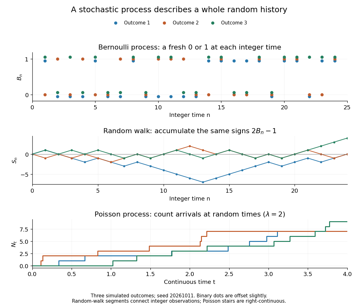
For the fair simple random walk on the integer line, the expected value is and the variance is . At time four, returning to zero requires exactly two positive steps, so . A rate-two Poisson process instead has . A single realized sample path does not establish either probability: they follow from the specified joint probability distributions.
The most revealing feature is often dependence. Two stochastic processes can have identical marginal distributions at every time while one forgets everything at the next step and the other repeats its first value forever. Their finite-dimensional distributions and covariance functions distinguish them. That extra structure is what makes a stochastic process useful for prediction.
The Borel-Cantelli lemmas turn a series of event probabilities into a statement about an entire infinite sequence of observations. A summable sequence of probabilities forces only finitely many occurrences almost surely, regardless of independence. A divergent series forces infinitely many occurrences when the events are mutually independent events. The precise event being measured is the limsup of events.
Imagine alarms with probabilities or , starting at . Both individual probabilities tend to zero. Nevertheless, the first alarm sequence eventually stops almost surely, whereas the second keeps returning almost surely if its events are mutually independent events. Reusing one uniform random variable for every alarm instead produces the shared-uniform counterexample to the second Borel-Cantelli lemma. Thus the individual probabilities alone do not determine long-run recurrence.
The main modes include almost sure convergence, convergence in probability, convergence in Lp, and convergence in distribution. The strong law of large numbers and weak law of large numbers explain why a sample mean approaches an expected value; the central limit theorem describes the probability distribution of its remaining error after magnification by .
Queueing theory studies how jobs accumulate while waiting for limited service: customers at a desk, requests at a computer, or calls competing for a connection. A queue model specifies how jobs arrive, their service times, the number of servers, the buffer size of a queue, and the service discipline. Its practical questions include the queue population, queueing delay, customer sojourn time, queue throughput, and server utilization.
Average spare capacity does not guarantee short waits. Even when the service rate of a queue exceeds the arrival rate, bursts of arrivals and unusually long service times can leave work waiting. The M/M/1 utilization and delay example shows that an 80 percent server utilization can turn a 12-minute mean service time into a 60-minute mean customer sojourn time. As capacity is approached, congestion grows sharply; reserving spare capacity can be much more valuable than its idle fraction suggests.
Two complementary ideas make queueing theory especially useful. Little's law converts a measured queue population and queue throughput into a mean customer sojourn time, using a counting identity rather than a particular arrival law. Poisson arrivals see time averages answers a different question: when do arriving customers see the same state frequencies as an observer sampling over time? That requires an exogenous Poisson process and a system that cannot anticipate its future arrivals. Neither result by itself determines all queueing delays; detailed models such as the M/M/1 queue and M/G/1 queue supply the remaining information.
A real-valued random variable is a measurable function from a probability space to the real numbers with their Borel sigma-algebra. More general targets give random elements. For every Borel set , measurability ensures that is an event, so the question "does the observed value lie in ?" has a defined probability.
The function is fixed; its input outcome is uncertain. This separates what we measure from how the uncertainty is modeled. A probability distribution is the resulting pushforward measure, . A cumulative distribution function, probability mass function, or probability density function describes that measure in an appropriate setting. The random variable and its probability distribution are different objects: the former also retains its relationship to other measurements on the same sample space.
For two independent uniform dice, let record their results and define and . The 36 ordered pairs are equally likely, but the resulting probability mass functions differ:For the sum, count the diagonal of the outcome grid having total . For the maximum, subtract the pairs with both results below from the pairs with both results at most . These examples show how a deterministic function transforms a simple input probability distribution into a nonuniform output one.
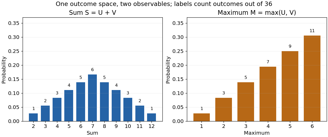


The corresponding expected values are and . The first follows immediately from linearity of expectation; the second follows from . Neither number must be an attainable result. An expected value describes an average under the probability measure, not a prediction that the next observation will equal it.
The distinction between a random variable and its probability distribution matters for dependence. and have the same discrete uniform distribution and are independent random variables. and a second copy of also have that same marginal probability distribution, but they always agree. Their joint probability distribution is concentrated on the diagonal; the marginals alone cannot say which relationship holds. This is why a model for several measurements must specify their joint law or an appropriate independence assumption.
Indicator random variables turn events into numbers: equals one on and zero elsewhere, and . This connects event counting with expected value and variance, and lets tools for random variables answer questions about probabilities. More complicated functions of observations can describe totals, waiting times, or estimation errors using the same framework.
The product measure is characterized on measurable rectangles depending on finitely many coordinates by the product of their component measures.
For a point uniformly distributed in the unit disk, its polar coordinates are independent with densities
A probability space is a measure space whose total measure is one. The sample space contains the elementary outcomes; the sigma-algebra contains the events to which the model assigns probabilities; the probability measure supplies those values. The sigma-algebra lets us combine observable questions using complements and countable unions while remaining within the model.
For two independent uniform dice, take , , and give each ordered pair mass . A random variable might record the sum, the larger result, or whether both results are even integers. These are different functions on the same sample space, rather than different elementary experiments. A probability distribution records the mass of the values of one such random variable and can forget information retained by the full probability space.
Percolation theory asks how many local connections must be available before a large connected structure appears. Start with a graph, randomly retain some edges or vertices, and study the resulting percolation clusters. In independent bond percolation, every edge is open with probability , independently of the others. In independent site percolation, the random decisions concern vertices instead. A percolation cluster is a connected component of a graph formed by the available connections; an open path joins two vertices exactly when they belong to the same percolation cluster.
The attraction is that a local rule can produce a global change. One open edge says little about travel across a large graph. Many alternative graph paths can nevertheless make distant connections likely. The model separates the geometry of possible connections from the probability distribution of which connections are usable. This was the central perspective of Broadbent and Hammersley's 1957 paper, which discussed porous solids and disease transmission as interpretations of the same mathematical structure: [ref]
https://courses.physics.ucsd.edu/2019/Spring/physics235/Broadbent_Hammersley.pdf. Percolation processes I: Crystals and mazes, introduction
. Independent bond percolation supplies a simplified model of those systems; the physical interpretation still requires justification of its independence assumptions.For a completely calculable example, consider the four edges around a square and ask whether opposite corners and are connected. There are two graph paths, each using two edges. Each open path has probability . Their events are independent events because the paths share no edges, even though they share endpoints. The inclusion-exclusion principle therefore givesAt , the connection probability is , larger than the for either chosen graph path. Counting all sixteen equally likely edge configurations gives the same answer: two configurations with exactly two open edges, four with three, and one with four connect to . Connectivity benefits from alternative routes; adding their probabilities without subtracting their overlap would count the all-open configuration twice.
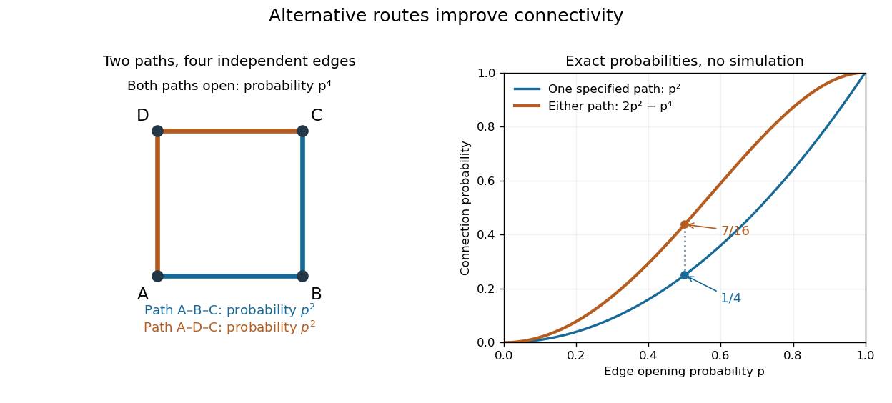
Two alternative paths increase the probability of connecting opposite corners
. Details. 
This finite calculation is already useful for studying redundant connections. The deeper question is what happens as the graph becomes arbitrarily large: does connectivity remain confined to finite percolation clusters, or can an infinite percolation cluster appear? The percolation probability and percolation critical probability make that question precise. A finite picture can illustrate the geometry, but cannot establish the existence of an infinite percolation cluster.
For every real ,For integer , strong induction proves this by splitting according to parity. If , every prime in divides , soIf , the valuation of a near-central binomial coefficient givesThe binomial estimates follow from the binomial theorem; in the odd case the two equal central coefficients together are at most . The result for real follows by replacing with .
There are unlisted articles, also show them or only show them.