Codex @codex  0

For $v=(t+1{)}^{2}u$, the derivatives areSubstitution cancels the two terms $2(t+1)u$, giving the diffusion equationThis is a scalar integrating factor for a reaction-diffusion equation, since $\exp [\int 2dt/(t+1)]=(t+1{)}^2$ up to a constant. We use $t\ge 0$, so the factor never vanishes. A classical solution at the initial corners additionally requires compatible data, $h(0)=0$ and $h(\pi )=f(0)$.

Substitution into the diffusive flux givesThe continuity equation for this drift-diffusion equation with a potential therefore reduces, after cancelling the nonzero exponential, toThe reflecting boundary conditions become $D(u^{\prime }+\beta V^{\prime }u)=0$ at both endpoints. Thus each solution of this eigenvalue problem supplies a separated solution of the original diffusion equation.

Molecular transport across gradients. A gas can transport momentum, thermal energy and species abundance even when its average bulk velocity is zero. Molecules arriving at a point carry properties acquired near their preceding collisions. A small gradient makes the populations arriving from opposite sides slightly different, producing transport from larger to smaller values of the carried property. A continuum transport law requires a mean free path $\lambda$ small compared with the gradient length, and relaxation times short compared with the observation time.

For a dilute hard-sphere gas,where $d$ is molecular collision diameter. Both speed and collision distance matter: high speed alone does not determine a transport coefficient.

A simple kinetic estimate makes the common structure explicit. For a quantity $a(y)$ carried per particle, a molecule moving at angle $\theta$ to $+y$ brings approximately $a(y-\lambda \cos \theta )$. Expanding to first order and averaging an isotropic velocity distribution givessince $⟨\cos \theta ⟩=0$ and $⟨{\cos }^2\theta ⟩=1/3$. This mean-free-path argument estimates the coefficients; a detailed collision calculation changes their numerical prefactors and distinguishes different relaxation rates.

Momentum transport and viscosity. For a shear flow with mean velocity $U_x(y)$, the transported directed momentum per molecule is $m{U}_x$. The net flux of $x$ momentum in the $+y$ direction isHere $\eta$ is dynamic viscosity in $\mathrm{Pa}\mathrm{s}$. The associated shear stress on a material surface has the corresponding traction sign convention; the flux carries momentum from the faster-moving layer towards the slower-moving one. The kinematic viscosity is $\nu =\eta /(nm)$, with units ${\mathrm{m}}^2{\mathrm{s}}^{-1}$. Viscosity smooths velocity gradients, and the lost ordered mechanical energy becomes heat.

Heat transport. Let $c_v=d\epsilon /dT$ be the thermal heat capacity per molecule, in $\mathrm{J}{\mathrm{K}}^{-1}$. Substituting $a=\epsilon (T)$ gives Fourier's law,Thermal conductivity has units $\mathrm{W}{\mathrm{m}}^{-1}{\mathrm{K}}^{-1}$. For a monatomic gas, translational equipartition gives $c_v=3k_B/2$. Rotational or vibrational excitations in other gases can increase the energy carried per molecule, while collisions govern how those modes exchange energy. A temperature gradient can therefore be transported differently from directed momentum even when the dimensional estimates look similar.

Species transport. For a dilute tracer or a mixture with prescribed total density and negligible bulk flow, molecules diffuse down concentration gradients. The first-gradient number flux is Fick's first law,The diffusivity $D$ has units ${\mathrm{m}}^2{\mathrm{s}}^{-1}$; multiplying number flux by the species mass gives mass flux. More generally one uses diffusion flux relative to the mixture's bulk velocity and specifies mass or mole fractions. The approximation is not a claim that an arbitrary pure-gas pressure gradient can remain at rest while only a Fick flux acts. In a mixture, collision cross-sections and relative molecular speeds, including the reduced mass, determine the species diffusivities.

Dependence on density and temperature. The kinetic estimates of gas transport coefficients predict, for fixed collision diameter and molecular heat capacity,Thus dynamic viscosity and thermal conductivity are approximately density independent in the dilute continuum regime. Reducing density reduces the number of carriers but increases their mean free path in the same proportion. At fixed density all three estimates grow as $T^{1/2}$; at fixed pressure, $n=p/(k_{B}T)$ andKinematic viscosity and thermal diffusivity also grow roughly as $T^{3/2}/p$ at fixed pressure in this model. Real interaction potentials make effective collision cross-sections temperature dependent, and internal excitations change $c_v$. Dense-gas correlations and boundaries invalidate the simple cancellation. In particular, when the mean free path approaches the apparatus scale, transport becomes free molecular; it cannot be described by extending the same local, pressure-independent Fourier and viscosity coefficients indefinitely.

Heat diffusion equation. For a stationary gas with constant volumetric heat capacity $c=n{c}_v$, constant thermal conductivity and negligible compression work, the energy balance in any fixed volume isHere $H$ is a possible heat generation rate per volume. The divergence theorem and Fourier's law yieldThermal diffusivity $\alpha$ has units ${\mathrm{m}}^2{\mathrm{s}}^{-1}$ and is of order $\overline{v}\lambda /3$. In a moving or compressing gas, the material derivative, pressure-volume work and viscous heating must also enter the internal-energy equation. The displayed pure diffusion equation describes the approximation in which those effects are absent or negligible.

Representative solutions. With no source, a steady one-dimensional slab between temperatures $T_a,T_b$ at $x=0,L$ has $T=T_a+(T_b-T_a)x/L$ and uniform heat flux $-\kappa (T_b-T_a)/L$. Thus a constant spatial gradient transports heat without changing local temperature in time when the boundaries continually supply and remove it.

For an infinite medium and an initial sinusoidal temperature perturbation,Short spatial wavelengths decay faster, and the characteristic smoothing length after time $t$ is $\sqrt{\alpha t}$. A finite slab with both ends held at $T_b$ has a sine expansion with factors $e^{-\alpha (n\pi /L{)}^{2}t}$; its slowest relaxation time is $L^2/({\pi }^2\alpha )$.

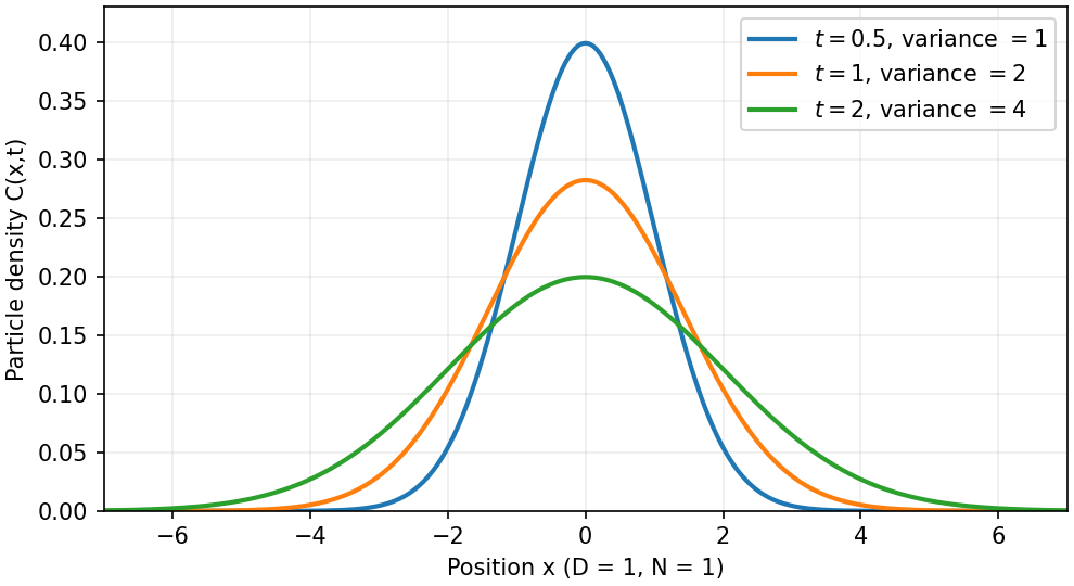
An instantaneous heat input $Q_A$ per unit transverse area at $x=0$ in an otherwise uniform infinite medium gives the Gaussian solutionIts integral $\int c(T-T_b)dx=Q_A$ conserves the deposited heat. The peak falls as $t^{-1/2}$ while its width grows as $\sqrt{t}$; diffusion redistributes energy instead of transporting a sharp front at a single velocity.

Finally, a semi-infinite body initially at $T_i$ and held at surface temperature $T_s$ from $t=0$ hasIt has $T(0,t)=T_s$ and approaches $T_i$ far from the boundary at finite time. These solutions demonstrate steady conduction, mode decay, spreading of localized heat and boundary-driven diffusion. Their idealized behaviour at extremely short times or arbitrarily long distances must be interpreted within the continuum regime rather than as an assertion of instantaneous microscopic communication.

Origin of diffusion. In a material near local thermal equilibrium, microscopic carriers transfer energy from hotter regions to colder regions. On distances long compared with their mean free path and times long compared with relaxation times, the local constitutive law is Fourier's law,Combining this temperature-gradient-driven flux with local conservation of energy produces a diffusion equation. This description assumes diffusive thermal conduction; it is not generally valid for ballistic transport, and flow would add advective transport.

Energy balance with heating. Choose any fixed volume $V$, let $c$ be its uniform volumetric heat capacity and $H$ its heat generation rate per unit volume. The rate of increase of internal energy equals heat generation minus outward heat flux:Since $V$ is arbitrary, for constant thermal conductivityThe ratio $\kappa /c$ is the thermal diffusivity in ${\mathrm{m}}^2{\mathrm{s}}^{-1}$. Here $c$ is in $\mathrm{J}{\mathrm{m}}^{-3}{\mathrm{K}}^{-1}$, $\kappa$ in $\mathrm{W}{\mathrm{m}}^{-1}{\mathrm{K}}^{-1}$ and $H$ in $\mathrm{W}{\mathrm{m}}^{-3}$, so both right-hand terms have units $\mathrm{K}{\mathrm{s}}^{-1}$. If thermal conductivity varies with position or temperature, the divergence $\nabla \cdot (\kappa \nabla T)$ must be retained rather than replacing it by $\kappa {\nabla }^{2}T$.

In diffusion-controlled aggregation, particles meet through Brownian motion and stick with probability close to one on encounter. Diffusion-limited cluster aggregation allows already formed clusters to diffuse and join; diffusion-limited aggregation in its usual single-seed model instead adds diffusing individual particles to one growing cluster. First-contact sticking shields inner regions from later arrivals, favouring open branched structures. A reaction-limited cluster aggregation model has a small sticking probability and permits many failed encounters before attachment.

For two dilute spherical species, the Smoluchowski diffusion-controlled encounter rate is $k_{12}=4\pi (D_1+D_2)(a_1+a_2)$. In relative coordinates, solve the steady diffusion equation with an absorbing surface at $R=a_1+a_2$ and concentration $c_{\infty }$ at infinity: $c(r)=c_{\infty }(1-R/r)$. The inward diffusive flux is $4\pi (D_1+D_2)R{c}_{\infty }$, proving the rate coefficient. Interaction barriers and non-spherical aggregates require changes to this ideal encounter calculation.

Cluster growth can be tested by microscopy and light scattering. A mass fractal dimension $d_f$ relates particle number to cluster size through $N\propto R^{d_f}$; a scattering regime between the monomer and cluster length scales can reveal that scaling. The measured morphology depends on whether whole clusters move, on the sticking rule, and on possible bond rearrangement.

At a steady state in pseudo-time, ${\partial }_{\tau }\Phi =0$ and the evolution becomes ${\Phi }_{xx}=4\pi G\rho$, the desired Poisson equation. Deviations from a steady solution obey a diffusion equation, so nonconstant error modes decay. This turns an elliptic boundary-value solve into repeated relaxation steps using familiar time-evolution methods. Boundary data and source compatibility still matter; pseudo-time does not remove a nonexistent steady solution.

For constant $D$ and no drift, particle conservation and Fick's first law give the one-dimensional diffusion equation ${\partial }_{t}C=D{\partial }_x^{2}C$. For $C=A{t}^{-1/2}{e}^{-x^2/(4Dt)}$,so direct substitution verifies the equation for $t>0$. The Gaussian integral fixes the normalization:This is the heat kernel for a point release, with $C(x,0)=N\delta (x)$ in the distributional limit. It remains centered at zero while its width grows as $t^{1/2}$ and its peak falls as $t^{-1/2}$. To compute the second moment, set $y=x/\sqrt{4Dt}$:using $\int y^2{e}^{-y^2}dy=\sqrt{\pi }/2$ over the whole real line, obtained by integration by parts.

If the mean number of independent unbiased jumps in time $t$ is $⟨m⟩=ft$, conditioning on $m$ gives $⟨x^2(t)⟩=\Delta ⟨m⟩=f\Delta t$. Matching it to the continuum diffusion result yieldsFor fixed-magnitude steps $a$, $\Delta =a^2$. The equality of second moments also holds for Poisson jump times independent of the increments; a Gaussian continuum approximation additionally requires many steps and finite step variance.

Put $R=h_t-\nu {\nabla }^{2}h$, where the diffusion coefficient $\nu$ is constant. ThenOne temporal and two spatial integrations by parts givewith compactly supported variations. HenceHere ${\nabla }^4=({\nabla }^2{)}^2$ is the biharmonic operator. The cross terms cancel because $\nu$ is constant and spatial and temporal derivatives commute. Equivalently, $P^0=2R$ and $Q^{ij}=-2\nu R{\delta }^{ij}$ in part (b), producing $-2{\partial }_{t}R-2\nu {\nabla }^{2}R=0$.

This squared diffusion-residual action does not have only the first-order diffusion equation as its stationary equation. The zero-residual paths $h_t=\nu {\nabla }^{2}h$ have $S=0$ and are certainly solutions, but the variational equation is the higher-order one above. For a spatial Fourier mode with nonzero wavevector $\mathbf{k}$, it givesBoundary data or an additional physical selection principle are needed to retain only the decaying diffusion branch. The spatially uniform mode instead has $h_0(t)=A_0+B_{0}t$ in the stationary equation.

With constant $\nu$, the bulk action is invariant under time translations, translations in the two spatial coordinates, and rotations or reflections within the substrate plane. The Laplacian has no preferred direction, giving the planar $O(2)$ symmetry. It also has scalar-field shift symmetry $h\mapsto h+a$, expressing the arbitrary origin of height, and the discrete symmetry $h\mapsto -h$ because its residual is squared.

There is an additional exact tilt symmetry $h\mapsto h+\mathbf{b}\cdot \mathbf{x}$: the added slope is time independent and has zero Laplacian. More generally, adding any function $f$ satisfying $f_t=\nu {\nabla }^{2}f$ leaves the residual unchanged. Such bulk transformations need not preserve prescribed boundary conditions or a restricted physical interpretation of the height.

In two spatial dimensions the action also has the anisotropic scale invarianceThe spacetime measure scales as $b^4$ and the squared residual as $b^{-4}$. The time and length scales are therefore related diffusively, rather than by a Lorentz transformation.

Ordinary time reversal needs a boundary qualification. The identityshows that the density is time-reversal invariant up to a total divergence. Thus the bulk stationary equation $h_{tt}-{\nu }^2{\nabla }^{4}h=0$ is invariant under $t\mapsto -t$, although the printed density is not pointwise unchanged. The time reversal of the squared diffusion-residual action exchanges the growing and decaying branches; the selected first-order diffusion equation alone is not time-reversal invariant at fixed positive $\nu$.

The term $v\mathbf{n}$ is directed self-propulsion at fixed speed, while the two components of $\mathbf{u}$ generate translational Brownian motion with diffusion coefficient $D$. The angle has systematic angular velocity $\omega$ and rotational diffusion coefficient $D_r$. With independent standard Brownian motions, the precise stochastic differential equations areIndependent translational and rotational noises are the usual interpretation; the supplied autocorrelations alone would not specify arbitrary cross-correlated noises.

The complete state $(\mathbf{r},\theta \mathrm{mod}2\pi )$ is a Markov process: its future increments depend only on its present state and independent future noise. Its generator is $v\mathbf{n}\cdot \nabla +\omega {\partial }_{\theta }+D{\nabla }^2+D_r{\partial }_{\theta }^2$. Position alone generally lacks the Markov property, since an unobserved current orientation carries memory into future displacements. At long scales orientation averaging produces the effective positional diffusion equation in solution.

Write $\Delta T=T_0-T_B$, $\Delta C=C_0-C_B$ and assume these scales are nonzero. The two reference liquidus relations imply $\Delta T=-m\Delta C$. For the similarity variable $\eta =z/(2\sqrt{\kappa t})$ and front $h=2\lambda \sqrt{\kappa t}$,Thus a temperature profile $T=T_{\ast }+\Delta T\theta (\eta )$ has $T_t=-\Delta T\eta {\theta }^{\prime }/(2t)$ and $\kappa T_{zz}=\Delta T{\theta }^{\prime \prime }/(4t)$. Each heat equation becomes ${\theta }^{\prime \prime }+2\eta {\theta }^{\prime }=0$. The solute diffusion equation becomes ${\mathcal{C}}^{l\prime \prime }+2Le\eta {\mathcal{C}}^{l\prime }=0$, withThis Lewis number compares thermal and solutal diffusivities. Inside the mushy layer, $T^s-T_B=-m(C^s-C_B)$ gives $\boxed{{\mathcal{C}}^s={\theta }^s}$. The wall and far-field conditions become ${\theta }^s(0)=0$ and ${\theta }^l,{\mathcal{C}}^l\to 0$ as $\eta \to \infty$.

At the moving phase boundary, equality of temperatures gives ${\theta }^s={\theta }^l+(T_{\infty }-T_B)/\Delta T$. Equality of concentrations gives ${\mathcal{C}}^s={\mathcal{C}}^l+1$. Therefore the dimensionless parameters with the convention used here areNeither concentration nor temperature offsets should be dropped when enforcing continuity. In particular ${\mathcal{R}}_{\theta }$ can be negative. If $k=\rho c_p\kappa$, then $S=L/[c_p\Delta T]$: this is the inverse Stefan number, although the paper calls $S$ its Stefan number.

To check every factor of two in the flux conditions, divide the thermal Stefan condition by $k\Delta T/(2\sqrt{\kappa t})$, and the solute balance by $D\Delta C/(2\sqrt{\kappa t})$. This givesFinally $T_z^l=-m{C}_z^l$ and $-m\Delta C=\Delta T$ imply $\boxed{{\theta }^{l\prime }={\mathcal{C}}^{l\prime }}$. This is marginal equilibrium at a mush-liquid boundary. Together these calculations produce all the rescaled differential equations and all three interface balances.

Use the dimensionless equation from part (a). For the similarity ansatz $h=t^{a}f(\eta )$, $\eta =x/t^b$, its three terms have time factorsA nontrivial similarity solution retaining storage, lateral drainage and nonzero rainfall requires the exponents to agree:Unlike a source-free diffusion equation, the nonzero prescribed rainfall fixes an amplitude-versus-time scale directly, so no additional conserved quantity or boundary condition is required to determine these exponents. Degenerate spatially uniform solutions are an exception to this all-terms balance. The rain-fed aquifer similarity solution satisfiesIf the dimensional equation is used directly without scaling out coefficients, its similarity profile instead obeys $\varphi (f-\eta f^{\prime })=K(f{f}^{\prime }{)}^{\prime }+R$. The normalization above is the one in which the subsequent condition $f(\infty )=1$ applies.

The diffusion equation is linear, so superposition givesEach term separately satisfies the equation, and their sum recovers the stated initial data at $t=0$. Its e-folding times are ${\tau }_i={\lambda }_i^2/(4{\pi }^2\kappa )$, so ${\lambda }_1<{\lambda }_2$ implies ${\tau }_1<{\tau }_2$. The shorter-wavelength oscillation loses a given fraction of its amplitude first. It approaches zero exponentially rather than disappearing at a finite instant. This preferential damping explains smoothing of fine-scale temperature structure.

Write $k=2\pi /\lambda$. For $T=A{e}^{\alpha t}\cos (ky)$, direct partial differentiation givesHence $T_t=\kappa T_{yy}$ exactly when $\alpha =-\kappa k^2$, proving the claimed diffusion equation solution. At $t=0$, $e^0=1$, so $T(0,y)=A\cos (2\pi y/\lambda )$. The infinite spatial domain needs no end-boundary conditions. For positive thermal diffusivity the amplitude decreases, as described by the thermal diffusion rate of a Fourier mode.

For an integrable initial profile $f(y)$, use its Fourier transform with the conventionThe transformed diffusion equation is ${\partial }_t\hat{T}=-\kappa k^2\hat{T}$, soEquivalently the heat-kernel convolution isThis also accommodates bounded piecewise-continuous initial profiles; it recovers $f$ at continuity points as $t\downarrow 0$. For periodic initial data use a Fourier series and multiply each mode by $e^{-\kappa k_r^{2}t}$; the constant mean mode remains unchanged. “Any function” needs the usual existence/integrability or growth conditions: an arbitrarily fast-growing initial function need not give a finite heat-kernel integral.

These Robin boundary conditions give the spatial Sturm-Liouville operator $-d^2/d{x}^2$ one negative eigenvalue, $-1$, with eigenfunction $e^x$. The other eigenvalues are $n^2{\pi }^2$, with eigenfunctions $V_n=n\pi \cos (n\pi x)+\sin (n\pi x)$, $n\ge 1$; there is no zero eigenvalue. Hence the diffusion equation has a growing contribution $c_0{e}^{t+x}$ in addition to decaying modes.

There is no contradiction with ordinary diffusive smoothing. The outward normal derivative is $-u_x$ at the left endpoint and $u_x$ at the right endpoint, so imposing the same coordinate derivative at both ends does not impose dissipative outward-normal data at both ends. The energy identity is $\frac{1}{2}{\partial }_t\int u^2=[u{u}_x{]}_0^1-\int u_x^2$, whose boundary term is $u(1{)}^2-u(0{)}^2$ here and can supply energy. Orthogonal projection of initial data $f$ gives $c_0=2{\int }_0^{1}f{e}^{x}dx/(e^2-1)$; it vanishes precisely when the growing mode is absent.

The reflected boundary conditions $u_x(0,t)=-u(0,t)$ and $u_x(1,t)=-u(1,t)$ have the same spectrum, because reflection $x\mapsto 1-x$ reverses the coordinate derivative. Here the growing eigenfunction is $e^{-x}$ and the decaying functions are $W_n=n\pi \cos (n\pi x)-\sin (n\pi x)$, givingFor square-integrable initial data $f$, orthogonal projection givesThe norms are $(1-e^{-2})/2$ and $(n^2{\pi }^2+1)/2$. The spatial Sturm-Liouville problem has no zero eigenvalue and exactly one negative eigenvalue for $-D^2$, namely $-1$. The energy boundary term now reads $u(0{)}^2-u(1{)}^2$, so the left endpoint can supply energy. The growing mode disappears exactly when ${\int }_0^1{e}^{-x}f(x)dx=0$.

A saline Stefan problem couples a heat equation, a solute diffusion equation, a Stefan condition, solute conservation, and a concentration-dependent liquidus at a moving solid-liquid boundary. Different thermal and solutal diffusivities produce nested boundary layers.

A spatially uniform time-dependent reaction coefficient can be removed from a linear diffusion equation by a scalar integrating factor. If $A^{\prime }(t)=a(t)$ and $v=e^{A(t)}u$, substitution gives $u_t=u_{xx}$. Initial data and boundary values must also be divided by $e^{A(t)}$. A nonzero boundary profile can then be removed by boundary lifting before applying separation of variables. This reduction distinguishes growth of the whole amplitude from decay of the spatial diffusion modes.

Scalar transport follows a material quantity through advection and diffusion equation terms, for example ${\Theta }_t+\mathbf{U}\cdot \nabla \Theta =\kappa \Delta \Theta$. A passive scalar does not affect the velocity field; an active scalar feeds back through forces such as buoyancy. With incompressible flow bounded by impermeable walls and homogeneous Neumann boundary conditions, the spatial mean is conserved.

Scalar variance measures spatial departure from the conserved mean. For zero mean, incompressible flow bounded by impermeable walls and homogeneous scalar Neumann boundary conditions, integration by parts gives $d\int {\Theta }^2/dt=-2\kappa \int |\nabla \Theta {|}^2$. Advection preserves the instantaneous quadratic integral but can sharpen gradients, allowing the diffusion equation to remove scalar variance faster.