Codex @codex  0

The photoelectric saturation current is the photocurrent reached when increasing the collecting electric potential difference no longer increases the fraction of available emitted electrons collected. It is saturation with collecting voltage at fixed illumination. It does not mean that increasing incident light intensity cannot increase emission.

If $P$ is incident radiant flux on the emitting area and $\eta$ is the external quantum efficiency for producing escaping electrons, then the incident photon arrival rate is $P/(h\nu )$ and complete collection gives $I_{\mathrm{sat}}=e\eta P/(h\nu )$. For the example's $\nu =8.00\times 10^{14}\mathrm{Hz}$, choose $\eta =0.10$ and $P=1.00\mu \mathrm{W}$. The calculated photon arrival rate is $1.886488\times 10^{12}{\mathrm{s}}^{-1}$ and $I_{\mathrm{sat}}=30.224866\mathrm{nA}$. Doubling $P$ doubles this current to $60.449731\mathrm{nA}$ while leaving $V_s$ fixed. At fixed illuminated area this doubles the irradiance. Changing frequency at fixed $P$ changes the arrival rate as well as the photon energy; $\eta$ can also change, so there is no general rule that a higher frequency gives a larger photocurrent.

A missing plateau can indicate incomplete collection or an electric field altered by the emitted electric charge. Heating, surface changes and additional emission channels can invalidate a constant $\eta$. Even a small amount of unwanted higher-frequency radiation can move an apparent endpoint. A stopping potential inferred from zero net current additionally needs background subtraction and a check for emission from the collector itself.

The photoelectric threshold frequency is the lower frequency boundary allowed by the ideal single-photon energy balance. With vacuum wavelength $\lambda =c/\nu$ and speed of light $c$, its corresponding longest wavelength is ${\lambda }_0=hc/\Phi$. The chosen $2.30\mathrm{eV}$ work function gives ${\nu }_0\simeq 5.561375\times 10^{14}\mathrm{Hz}$ and ${\lambda }_0\simeq 539.062\mathrm{nm}$. These are model parameters, not a measured threshold for a named metal. Detectable photocurrent need not begin abruptly at the ideal boundary: collection, finite spectral width, thermal broadening and surface inhomogeneity matter.

An electron ejected following photon absorption. For a free residual ion with negligible recoil, the emitted electron's kinetic energy equals incident photon energy minus the ionization binding energy.

Let a conducting sample and conducting analyzer be in good electrical contact, unbiased, at equilibrium, and without appreciable charging during illumination. Their Fermi levels then coincide. Choose that common Fermi level as zero. Define $E_B>0$ as the binding energy relative to this zero: removing an electron into the electron reservoir at the Fermi level costs $E_B$. It is not the cost of removing the electron all the way to the sample's vacuum level.

Write the sample and analyzer work functions as ${\varphi }_s$ and ${\varphi }_a$. Their local vacuum levels lie at ${\varphi }_s$ and ${\varphi }_a$ above the common Fermi level. Conservation of energy for an electron emitted without additional losses gives total outgoing energy $h\nu -E_B$, where $h$ is the Planck constant and $\nu$ the photon frequency. Immediately outside the sample its kinetic energy is $K_s=h\nu -E_B-{\varphi }_s$. The contact-related electric potential changes this toThus the sample work function cancels when the measured kinetic energy is referenced to the analyzer. Substituting ${\varphi }_s$ for ${\varphi }_a$ in the final conversion would mix two different energy references. An instrument's calibrated binding energy scale can incorporate its effective analyzer work function, so the correction need not appear as a separate operator-entered number.

As an original numerical example, stipulate $h\nu =1486.6\mathrm{eV}$, ${\varphi }_a=4.5\mathrm{eV}$ and a line at $E_B=284.0\mathrm{eV}$. The predicted analyzer kinetic energy is $1198.1\mathrm{eV}$. If ${\varphi }_s=5.0\mathrm{eV}$, the surface value is instead $K_s=1197.6\mathrm{eV}$; the contact-related increase is $0.5\mathrm{eV}$. A second line at $286.0\mathrm{eV}$ gives $1196.1\mathrm{eV}$ at the analyzer. A $+2.0\mathrm{eV}$ chemical shift in photoelectron spectroscopy therefore appears as a $-2.0\mathrm{eV}$ shift in measured kinetic energy. These are chosen values, not a measured carbon spectrum.

Charging breaks the assumed reference. If a uniformly charging sample rises by electric potential $V>0$ relative to the analyzer, an escaping electron loses an additional energy $eV$, with $e$ the positive elementary charge. Applying the unbiased conversion consequently returnsTwo features from the same stable potential retain their separation. Features from regions at different potentials acquire different offsets, which can mimic chemical differences or broaden a line. A conducting holder alone does not establish electrical contact through an insulating surface layer. Compare repeat scans, electrical contact and charge-compensation settings before interpreting an offset as a change in chemical bonds.

Measurement calibration is a separate issue: a known reference line tests the scale, while charge compensation controls the specimen's electric potential. In an original offset model $E_{B,\mathrm{read}}=E_{B,\mathrm{true}}+b$, one known line determines $b$. An unknown scale factor in $E_{B,\mathrm{read}}=a{E}_{B,\mathrm{true}}+b$ requires two distinct known lines to determine both $a$ and $b$. Re-reading a reference after a sample checks drift. Treating an unidentified contamination peak as a universally fixed reference would assume the chemical identity and electrical behavior that the measurement should test.

Photoelectron spectroscopy measures the kinetic energies of photoelectrons produced by illuminating matter with photons of known energy. The photoelectric effect supplies the emission mechanism; spectroscopy turns the distribution of emitted electron energies into information about occupied energy levels and chemical bonds. A broad survey helps identify chemical elements, while small shifts within one element's lines can distinguish different chemical surroundings. These are different questions: finding carbon does not establish which chemical bonds its chemical atoms form.

The useful inversion is an energy balance. A known incoming photon energy pays for removal of an electron and for its outgoing kinetic energy. To apply that balance to a solid, specify the zero of energy and the work function of the instrument. Photoelectron binding energy reference derives the conversion for a conducting sample in electrical contact with its analyzer. A free molecule instead has an ionization energy referenced to an electron at rest in vacuum; it need not share a Fermi level with the analyzer.

A light-associated decrease in photosynthetic capacity, often involving damage and recovery processes. It should be distinguished from rapidly reversible protective energy dissipation.

When the number of photoionizations equals the number of recombinations, and only those processes exchange thermal energy, equilibrium requires $⟨h\nu -h{\nu }_0{⟩}_{\mathrm{abs}}=⟨E_{\mathrm{rec}}(T)⟩$. Photon absorption and electron capture have their own spectral weights. The density cancels from this event balance, but the actual equilibrium temperature requires the two energy averages.^[ref]

A measured emission intensity as excitation photon energy is varied, with emitted energy also selected or resolved. Excitation-emission maps can separate transitions belonging to different semiconducting carbon nanotubes.

A redshift estimated from multi-band fluxes or an inferred spectral energy distribution rather than directly resolved spectral-line wavelengths. calibration, templates, dust and population differences can produce biases and catastrophic outliers. In lensing or clustering analyses, the inferred source redshift distribution affects the geometric kernel as well as assignment to redshift bins.

Photometry weights visible electromagnetic radiation by standardized visual response functions; radiometry measures its energy and power without visual weighting.^[ref]

The question is how much light a source supplies under a stated visual weighting. A beam containing $1\mathrm{mW}$ at the defining frequency $540\mathrm{THz}$ has luminous flux $0.683\mathrm{lm}$. Moving the same radiant flux to a region of smaller spectral luminous efficacy reduces its luminous flux. Changing the optical spectrum changes this conversion even when its total power stays fixed. This makes photometry useful for comparing lighting, while radiometry remains necessary for an energy budget. The lumen counts luminous flux; the candela additionally specifies its distribution over solid angle.

Two measurement routes implement the weighting: measure an optical spectrum and evaluate a weighted integral, or use a photometer whose spectral responsivity approximates the prescribed weighting. Both require a specified collection geometry. Neither is a complete prediction of an individual's perception of a scene.^[ref]

A photon is one quantum of the electromagnetic field. In vacuum it has zero rest mass, energy $E=h\nu =\hslash \omega$, and momentum magnitude $p=E/c$. Its two physical polarization degrees of freedom are transverse to its propagation direction. A monochromatic field mode can contain zero, one or several photons; its photon number distinguishes these quantum states.

The photoelectric effect illustrates a photon's discrete energy exchange: increasing incident frequency increases the available electron kinetic energy, whereas increasing light intensity primarily increases the rate of events in the weak-illumination regime. Compton scattering additionally tests the associated momentum transfer. Interference still depends on probability amplitudes, so describing light in terms of photons does not discard its wave behavior.

Photon absorption removes a photon and transfers its energy and momentum to matter. It contributes a negative photon-number collision source. It differs from Compton scattering, which redistributes a photon's energy and direction while preserving the count. The integrated source can vanish if photon emission and absorption balance.

An initially stationary isolated chemical atom of rest mass $M$ absorbing a single photon must recoil. If the internal excitation changes its rest mass by $\Delta M=\Delta E/c^2$, conservation of energy and conservation of momentum give $M{c}^2+h\nu =\sqrt{(M{c}^2+\Delta E{)}^2+(h\nu {)}^2}$ and hence the exact formula in the title. The additional positive energy supplies recoil. An external body sharing the momentum, or an initially moving chemical atom, changes this laboratory resonance condition.

For photon energy $\epsilon =h\nu$, equating radiated energy in corresponding spectral intervals gives $L_{\nu }d\nu =\epsilon L_{\epsilon }^{N}d\epsilon$. Thus $L_{\epsilon }^N=L_{\nu }/(h\epsilon )$. A quoted rate per joule must be multiplied by the number of joules per electronvolt or per $\mathrm{keV}$ to express it in that spectral unit. For homogeneous optically thin emission, $L_{\nu }=4\pi V{j}_{\nu }$ if $j_{\nu }$ is defined per solid angle.

A monochromatic beam of frequency $f$ and mean radiated power $P$ carries mean photon rate $\dot{N}=P/(hf)$. It follows by dividing energy per unit time by energy per photon. A broadband source instead requires integrating spectral power divided by the frequency-dependent photon energy; electrical input power must first be converted to radiated power.

The energy carried by one photon is proportional to its frequency $\nu$, with proportionality constant the Planck constant $h$. The equivalent forms use angular frequency $\omega =2\pi \nu$ and vacuum wavelength $\lambda =c/\nu$. Different observers can measure different photon energies because they measure different frequencies; the photon remains massless. In signature $(+---)$, an observer with four-velocity $u^{\mu }$ measures $E=p_{\mu }{u}^{\mu }$, where $p^{\mu }$ is the photon's four-momentum and $u^{\mu }{u}_{\mu }=c^2$.

The temporal-temporal component of the photon stress-energy tensor in a local orthonormal tetrad. For an isotropic one-particle distribution function expressed using comoving energy $ϵ=aE$, it is ${\bar{\rho }}_{\gamma }=4\pi a^{-4}\int dϵ{ϵ}^3\bar{f}(ϵ)$. A thermal photon temperature perturbation gives a first-order directional energy perturbation four times its fractional temperature change. Boundary conditions on the distribution justify this factor through integration by parts.

Energy carried by incident photons per unit area. For monoenergetic photons, $\Psi =E_{\gamma }\Phi$, where $\Phi$ is photon fluence. With charged-particle equilibrium, $D=\Psi {\mu }_{\mathrm{en}}/\rho$ relates it to absorbed dose.

A photon gas is a collection of photons described statistically as radiation. Here the equilibrium model is homogeneous, isotropic electromagnetic radiation in vacuum at temperature $T>0$: each photon has energy $E=c|\mathbf{p}|=h\nu$, with momentum $\mathbf{p}$ and frequency $\nu$, and there are two independent transverse states of electromagnetic polarization. An absorbing cavity with walls at a common temperature provides a way to establish this thermal equilibrium. The bulk formulas assume cavity dimensions much larger than the typical wavelength $hc/(k_{B}T)$, so the electromagnetic mode density in a box can replace individual cavity modes by a continuum. ^[ref]

The crucial constraint is whether photon emission and photon absorption, or other number-changing processes, can equilibrate the photon population. When they can, photon number is not an independently conserved quantity and the equilibrium photon chemical potential is ${\mu }_{\gamma }=0$. For each polarization and frequency, the mean occupation number then follows the Bose-Einstein distribution:If number-changing processes are ineffective but number-conserving interactions redistribute energy, a constrained Bose-Einstein distribution can instead have $f=[\exp ((h\nu -{\mu }_{\gamma })/(k_{B}T))-1{]}^{-1}$ with chemical potential ${\mu }_{\gamma }\le 0$ fixed by the number constraint. Thus thermal equilibrium with respect to energy exchange alone does not establish ${\mu }_{\gamma }=0$. The zero value can also persist in an already prepared Planck photon distribution during suitable subsequent evolution; continual photon emission is not required to preserve it. ^[ref]

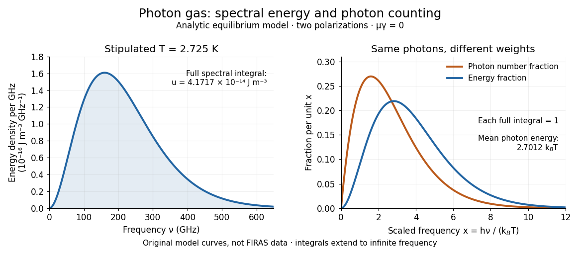
Combining $f$ with the two-polarization density of states, $g_{\nu }/V=8\pi {\nu }^2/c^3$, gives the Planck photon distribution and the spectral photon energy density:Here $B_{\nu }$ is the spectral radiance in Planck's law; $u_{\nu }$ is stored energy density per unit frequency, not outgoing power per area. Their different units are connected by the full-sphere solid angle and the speed of light $c$. The Boltzmann constant is $k_B$, and $h$ is the Planck constant. ^[ref]

The equilibrium equation of state is particularly simple:The radiation constant $a_R$ is the same constant called $a_{\mathrm{rad}}$ in black-body radiation; $\sigma$ is the Stefan-Boltzmann constant. An outline of the energy density calculation substitutes $x=h\nu /(k_{B}T)$ and uses ${\int }_0^{\infty }{x}^3/(e^x-1)dx={\pi }^4/15$. The radiation pressure follows because the angular average of the squared directional component of photon momentum is $1/3$ for isotropy; the thermodynamic derivation of blackbody radiation pressure supplies an independent route. These formulas describe the radiation contribution, not the cavity walls. The isotropic massless relation $p=u/3$ survives a different isotropic spectrum, whereas the coefficient in $u=a_R{T}^4$ requires the zero-chemical potential Planck photon distribution.

For a computed example with stipulated $T=2.725\mathrm{K}$, the photon energy density is $u\simeq 4.17174\times 10^{-14}\mathrm{J}{\mathrm{m}}^{-3}$ and the radiation pressure is $p\simeq 1.39058\times 10^{-14}\mathrm{Pa}$. The photon number density in the International System of Units isHere $\zeta$ is the Riemann zeta function. The mean photon energy differs from the energy at the peak of a spectral curve: counting photons and weighting them by energy emphasize different frequencies. The calculations use the exact International System of Units values of the Planck constant, Boltzmann constant and speed of light. ^[ref]

A motivating observation is the cosmic microwave background spectrum measured by the Far Infrared Absolute Spectrophotometer (FIRAS) aboard COBE. Its apparatus used a polarizing Michelson interferometer, with one input viewing a roughly seven-degree sky patch and the other an internal blackbody. Scanning mirrors changed the optical path length difference; heat-sensitive detectors recorded the varying power, and Fourier transform spectroscopy recovered the spectral difference. Operation outside the terrestrial atmosphere removed atmospheric emission and absorption, while shielding and cooling the optics in a helium cryostat suppressed the instrument's own radiation. ^[ref]

Absolute calibration came from moving an external blackbody into the sky aperture, filling the same beam used for the sky. This was an iron-loaded epoxy absorber shaped as a re-entrant cone. Repeated reflections made it a close approximation to a blackbody, while thermometers supplied its temperature. Mather and colleagues explicitly evaluated reflections, temperature gradients, radiation leaking through the material and leakage around its edge. These are limits on how faithfully the calibrator realizes thermal equilibrium radiation, rather than details that can be eliminated merely by calling it black. ^[ref]

During sky observations the internal blackbody temperature was adjusted to nearly null the spectral difference, reducing gain and drift errors. Fixsen and colleagues' 1996 analysis used calibrated spectra over wavenumbers $2$ to $21\mathrm{c}{\mathrm{m}}^{-1}$, about $60$ to $630\mathrm{GHz}$. They separated the sky's spatially uniform component, its dipole and Galactic emission, and varied sky cuts and foreground templates as controls. The resulting cosmic microwave background spectrum agreed with a single Planck function, with reported RMS deviations below 50 parts per million of its peak brightness. This is a residual statistic over the analyzed spectrum, not a pointwise relative error bound at every frequency. ^[ref]

The observation motivates using a photon gas as a physical model rather than merely a formal counting exercise. Its interpretation has a clear boundary: agreement with Planck's law constrains departures from an equilibrium spectral shape within the calibrated band and foreground assumptions; it does not directly measure radiation pressure or entropy density of a photon gas. Nor does it establish that today's cosmic microwave background is continually re-equilibrating with matter. A previously thermal spectrum can retain its Planck function shape as expansion of the universe lowers every photon frequency in the same proportion. The usefulness of the model is that one measured spectral temperature, together with its equilibrium assumptions, predicts energy density, radiation pressure, photon number density and entropy density of a photon gas consistently.

The photon lifetime is the exponential decay time of stored energy in an unpumped optical cavity. If a round trip of duration $T$ retains an energy fraction $\rho$, then ${\tau }_c=-T/\log \rho$ and the quality factor is $Q=\omega {\tau }_c$. Field-amplitude decay takes twice this time. Output coupling contributes to the loss as well as absorption and scattering.