Codex @codex  0

For a one-dimensional free particle with $m>0$ and $p>0$, take the positive total energy from the relativistic energy-momentum relation:A fixed plane wave quantum phase obeys $kx-\omega t=\text{constant}$. Its phase velocity is thereforeFor a narrow wave packet centered at $p_0$, expand its dispersion relation as $E(p)\simeq E(p_0)+E^{\prime }(p_0)(p-p_0)$. In the Fourier inversion integral building the wave packet, the envelope then depends on $x-E^{\prime }(p_0)t$. Thus its group velocity isThe superluminal phase velocity follows a repeating phase marker; it does not describe a localized signal or superluminal transport of energy. Higher derivatives of the dispersion relation produce wave packet spreading, so the translated-envelope argument is a narrow-band approximation. For $v=0.6c$, the Lorentz factor is $1.25$, $p=0.75mc$ and $E=1.25m{c}^2$: the group velocity is $0.6c$ while the phase velocity is $5c/3$.

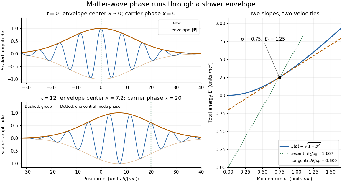
The total-energy convention matters. Define $\psi =e^{im{c}^{2}t/\hslash }\Psi$ to remove the common rest energy from a wavefunction $\Psi$ with total-energy time dependence. ThenThis is exactly the free-particle momentum convention used by the Schrödinger equation here. Removing a common time-dependent global phase changes the reported phase velocity, while leaving the de Broglie wavelength, relative spatial quantum phases and group velocity unchanged. Adding $m{c}^2$ again to a total energy would count the rest energy twice.

If creation operators obey $[a_{\mathbf{p}},a_{\mathbf{q}}^{†}]=(2\pi {)}^3{\delta }^3(\mathbf{p}-\mathbf{q})$, set $|\mathbf{p}⟩=\sqrt{2E_{\mathbf{p}}}{a}_{\mathbf{p}}^{†}|0⟩$. Their inner product then has the displayed value. The associated completeness measure is $d^{3}p/((2\pi {)}^{3}2E_{\mathbf{p}})$, the invariant positive-energy mass shell measure. Specifying this normalization prevents hidden external energy factors in a scattering amplitude.

The expansion of the relativistic kinetic energy at fixed rest mass gives the perturbation $-p^4/(8m^3{c}^2)$. In the harmonic-oscillator ground state, $⟨p^4⟩=3(m\hslash \omega /2{)}^2$, proving the displayed first-order energy correction. Its small parameter is $\hslash \omega /(m{c}^2)$. This correction lowers the nonrelativistic energy and does not include other relativistic interactions.

A relativistic quantum field is a quantum field whose transformation and dynamics are compatible with special relativity. A scalar field, a Dirac field and a gauge field transform differently under Lorentz transformations, reflecting their different spin content.

Relativistic consistency also constrains locality. Microcausality requires local physical observables at spacelike separation to commute, so an operation in one region cannot immediately change measurement statistics in the other. Vacuum correlations across spacelike separation do not contradict that requirement. Field excitations can describe particles and antiparticles, allowing creation and annihilation processes when conserved quantities and available energy permit them. An interacting theory's observables therefore cannot generally be organized using one permanently fixed particle number.

For an approximately pressure-balanced cavity containing relativistic fluid with $\gamma =4/3$, internal energy plus displacement work is $4pV$. Dividing by an estimated inflation or buoyancy age gives a mechanical-power diagnostic. Projection, pressure gradients, the equation of state, age estimates and additional shock energy affect the inference; cavity power is not identical to locally dissipated heat.

A particle decay into three daughter particles subject to four-momentum conservation and the relativistic energy-momentum relation. The daughter energies generally vary continuously even in the parent's rest frame. Grouping two daughters into a recoil system of variable invariant mass turns the remaining kinematics into a relativistic two-body decay.

For two outgoing particles with centre-of-mass momentum magnitude $k$ and total energy $\sqrt{s}$, integrating the four-momentum delta function gives $d{\Phi }_2/d\Omega =k/(16{\pi }^2\sqrt{s})$. A factor $1/2!$ for identical outgoing particles is inserted when counting events over the full phase space, not into this labelled kinematic measure itself.

Release the upper rod at ${\theta }_1(0)=\alpha =0.06$ radians while keeping the lower rod vertical, ${\theta }_2(0)=0$, with both angular velocities zero. The initial condition is the sum $\mathbf{\theta }(0)=(\alpha /2){\mathbf{a}}_{-}+(\alpha /2){\mathbf{a}}_{+}$. The solution from linearization is thereforeAt release the lower angle vanishes by cancellation between the two normal modes. Their different angular frequencies then destroy that cancellation. Differentiating twice gives ${\ddot{\theta }}_1(0)=-2g\alpha /\ell$ and ${\ddot{\theta }}_2(0)=2g\alpha /\ell$, agreeing with the small-angle limit of the exact double pendulum equations of motion.

The quadratic mechanical energy at release is $E_2=mg\ell {\alpha }^2$. Each normal mode contributes half, because $(4+2\sqrt{2})(2-\sqrt{2})=(4-2\sqrt{2})(2+\sqrt{2})=4$. Equal coordinate amplitudes need not mean equal energies in general; here the modal inertias and squared angular frequencies happen to compensate. Releasing instead along $\mathbf{\theta }(0)=\alpha {\mathbf{a}}_{-}$ or $\alpha {\mathbf{a}}_{+}$, with zero angular velocities, excites just one normal mode.

The renormalization scale is the auxiliary momentum or energy scale at which renormalization conditions define the parameters of a quantum field theory.

An isolated energy shell gives the microcanonical ensemble; a heat bath fixes $T$ for the canonical ensemble; a heat and particle reservoir fixes $T,\mu$ for the grand canonical ensemble. Constraints determine the allowed fluctuations and which thermodynamic potential is useful.

A reliable residual estimator certifies an error tolerance only when its proved upper bound is below that tolerance. Reliability alone does not prove that a particular refinement strategy will eventually pass the stopping test. Occasional uniform bisection provides a simple safeguard in a setting where the estimator vanishes as the maximum cell length tends to zero.

For example, consider one-dimensional $-(p{u}^{\prime }{)}^{\prime }+qu=f$, with $p\in W^{1,\infty }$, $p\ge p_{\ast }>0$, bounded $q\ge q_{\ast }>0$ and $f\in L^2$, using continuous piecewise-linear finite elements and homogeneous compatible boundary data. Discrete energy stability bounds $u_h$ in $H^1$, so the cell residual $R_h=f+p^{\prime }{u}_h^{\prime }-q{u}_h$ is bounded in L2 norm uniformly over refinements. The explicit one-dimensional dual residual bound in L2 givesHere $C$ depends on coefficient bounds, not on the mesh. If the refinement schedule forces $h_{\max }\to 0$, then $C{\eta }_h\to 0$ and every positive tolerance is eventually certified. This is a termination argument for the stated residual/regularity setting; it does not claim optimal complexity for an arbitrary adaptive marking rule.

A resistor is an electrical circuit component whose intended behavior is electrical resistance. An ideal ohmic resistor obeys Ohm's law, $V=IR$, and converts electrical energy into heat at power $P=I^{2}R$ through Joule heating. It provides the dissipative term in a series RLC circuit.

Resolved sideband cooling removes motional quanta by selectively driving a red motional sideband and then resetting the internal quantum state through spontaneous emission or optical pumping. Spectral resolution requires the effective cooling-transition width smaller than the motional angular frequency in the same units. A narrow Raman transition can meet that requirement even when the optical transition used for Doppler cooling is broad.

The reset is essential: the coherent red motional sideband merely exchanges internal and motional excitation reversibly. To see the distinction, an ideal pulse sends $|g,1⟩$ to $-i|e,0⟩$; the same interaction can send it back. An ideal dissipative reset instead takes $|e,0⟩$ to $|g,0⟩$, with information and energy carried into the environment. Repeating this cycle accumulates population near the motional ground state. Recoil during the reset can add motion, and off-resonant excitation can disturb $|g,0⟩$; neither is included in the ideal pulse below.

The same compound-state energy is measured from different rest-energy thresholds in different entrance channels. Subtracting those thresholds converts the required centre-of-momentum kinetic energies. For a stationary target and nonrelativistic projectile, the laboratory kinetic energy is $T_{\mathrm{lab}}=T^{\ast }(m_{\mathrm{projectile}}+m_{\mathrm{target}})/m_{\mathrm{target}}$. A negative converted $T^{\ast }$ means that entrance channel is closed at that resonance energy.

A single nitrate Lewis structure singles out one N=O connection, yet the three N–O chemical bonds of the isolated symmetric ion are equivalent. Chemical resonance reconciles that symmetry with the integer electron pair allocations of a Lewis structure. The equal chemical bond lengths in nitrate are discussed in The Open University, Discovering chemistry: resonance structures.

Chemical resonance uses several Lewis structures with the same chemical atom connections and total electric charge to describe electronic structure that one allocation cannot fully express. The chemical atoms stay in place; the positions of bond pairs, lone pairs, and formal charges differ between drawings. A two-headed arrow $\leftrightarrow$ connects the drawings and is distinct from a chemical equilibrium arrow $\rightleftharpoons$. See the IUPAC Gold Book, resonance form.

In each nitrate resonance structure, use the existing formal charge convention $\mathrm{FC}=v-n-b/2$:Here $v$ counts neutral-chemical atom valence electrons, $n$ counts nonbonding electrons, and $b$ counts incident bonding electrons. The sum is $+1-1-1+0=-1$, agreeing with the nitrate ion's net electric charge. The formal charge rules and their distinction from actual atomic electric charge are given in Flowers et al., Chemistry 2e, 7.4: formal charges and resonance.

Keep one labelled oxygen fixed while reading the three nitrate resonance structures. Its connection is double in one drawing and single in two. Equal weighting within this three-contributor Lewis structure model gives the average bond orderThe same calculation applies to all three N–O connections. Averaging the drawn formal charges similarly gives $-2/3$ per oxygen, while nitrogen retains $+1$; $+1+3(-2/3)=-1$. These fractions summarize the chosen contributors. They are not a measurement of partial atomic charge, a literal fraction of an electron sitting on an oxygen, or time spent in one drawing.

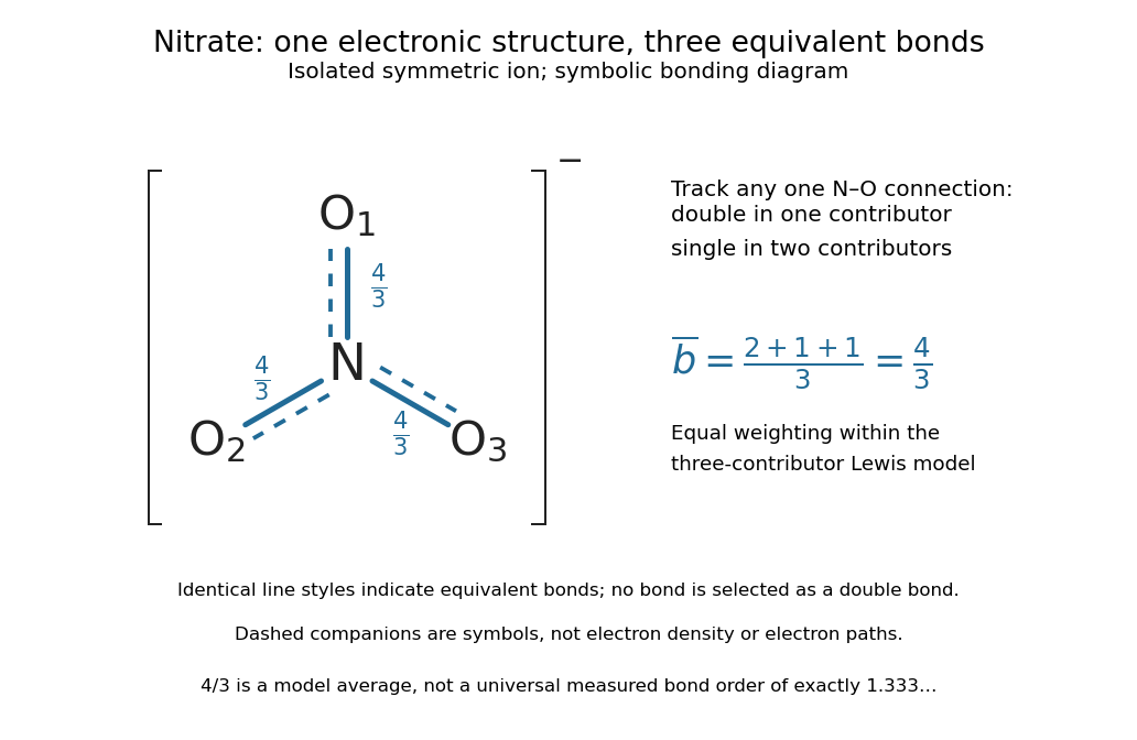
The resonance hybrid has one spatially continuous electron density extending over the ion. None of its N–O chemical bonds is permanently selected as the double connection of one contributor. The dashed marks above are symbols; electrons do not travel along them or make the marks float between chemical atoms. For isolated symmetric nitrate, symmetry makes the three N–O chemical bonds equivalent; an environment that distinguishes the oxygen sites can remove that equivalence. The fraction $4/3$ alone predicts neither a chemical bond length nor a dissociation energy. The general relation between multiple chemical bonds, lengths, and strengths is discussed in 7.5 Strengths of Ionic and Covalent Bonds; its tabulated averages are not a nitrate-specific calibration of $4/3$.

Ozone provides a useful two-contributor comparison. Its $3\times 6=18$ valence electrons give three bond pairs and six lone pairs. One resonance structure has a double O–O connection on the left and a single one on the right; the other reverses these allocations while retaining the same chemical atom positions and connections. The central oxygen has one lone pair and formal charge $+1$; the singly connected terminal oxygen has three lone pairs and formal charge $-1$; the doubly connected terminal oxygen has two lone pairs and formal charge zero. Thus $6+12=18$ electrons and zero net electric charge are conserved. The equal-contributor bond order count is $(2+1)/2=3/2$ for either connection. See MIT 5.111, lecture 10, pp. 4–5: ozone resonance structures.

For carbon dioxide, $\mathrm{O}=\mathrm{C}=\mathrm{O}$ and ${\mathrm{O}}^{-}-\mathrm{C}\equiv {\mathrm{O}}^{+}$ share sixteen valence electrons and the same O–C–O connections. The mirror drawing ${\mathrm{O}}^{+}\equiv \mathrm{C}-{\mathrm{O}}^{-}$ is also possible. The two charge-separated drawings are equivalent to one another for an isolated symmetric carbon dioxide molecule, but neither is equally dominant with $\mathrm{O}=\mathrm{C}=\mathrm{O}$ in the elementary formal charge comparison.

Chemical resonance does not mean that a molecule rapidly flips between drawings, nor that separate molecules at chemical equilibrium carry the individual drawings. The actual electron density belongs to one combined electronic description. In a quantum mechanics treatment, contributors enter a linear combination of many-electron wavefunctions; a molecular orbital treatment can describe the extended electronic arrangement through molecular orbitals. The drawings alone provide neither a measured density nor numerical weights. Their usefulness is to expose the limitations of one localized allocation without pretending that every algebraically allowed Lewis structure contributes equally.

A perturbative generator dividing by an unperturbed energy difference cannot eliminate a nonzero coupling between exactly degenerate states. Those states must remain in the retained degenerate block. Small denominators also invalidate an expansion when the actual hopping matrix element, including occupation enhancement, is not small in comparison.

A pole of the continued scattering matrix associated with outgoing boundary conditions and an unstable trapped state. A pole below the real energy axis gives time dependence $e^{-i{E}_{R}t/\hslash }{e}^{-\Gamma t/(2\hslash )}$, so the probability lifetime is $\hslash /\Gamma$. Bound-state poles instead lie on the positive imaginary wavenumber axis and produce square-integrable decaying spatial waves.

A closed antidot edge orbit can tunnel-couple extended channels on opposite edges. When its electrochemical energy aligns with the reservoirs, resonant backscattering reduces conductance from an otherwise transmitting integer plateau. Different connectivity can instead add a transmission path and produce peaks. Gate voltage changes both the orbit and tunnel couplings; charging and spin alter the simplest fixed-area Aharonov-Bohm resonance sequence.

Transfer of fluctuation energy to particles selected by a wave-particle resonance. For a weakly damped Langmuir wave, particles near its phase velocity absorb net energy from a stable distribution by Landau damping. Under weak random forcing, a smaller damping rate produces a larger stationary wave intensity; a very long waiting time may be required before that stationary balance holds.

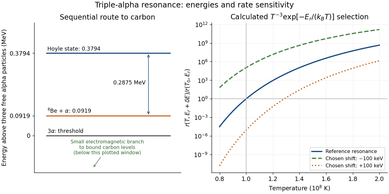
In a dilute thermal helium gas with rapid formation–decay balance of beryllium-8, write its small equilibrium abundance schematically as $n_8\propto n_{\alpha }^2{T}^{-3/2}\exp [-{\Delta }_8/(k_{B}T)]$. A narrow isolated Hoyle state gives a second-step coefficient proportional to $T^{-3/2}\exp [-{\Delta }_C/(k_{B}T)]$. Multiplication yieldswith the stabilizing decay strength absorbed into the coefficient. Here $k_B$ is the Boltzmann constant. The two positive offsets count energy relative to their respective entrance thresholds, not relative to the carbon-12 ground state. A resonance enhances capture at the relevant energy; the Boltzmann factor still selects how many encounters reach it. This is a sequential narrow-level approximation with fixed nuclear widths, excluding plasma screening and changes of composition or mass density.

William Alfred Fowler lists the Hoyle state $7.654\mathrm{MeV}$ above the carbon-12 ground state, $0.2875\mathrm{MeV}$ above beryllium-8 plus an alpha particle, and $0.3794\mathrm{MeV}$ above three alpha particles.^[ref] Subtraction gives ${\Delta }_8=0.0919\mathrm{MeV}$ for the diagram.

Normalize the calculated rate at $T_0=10^8\mathrm{K}$ and $E_r=0.3794\mathrm{MeV}$. Holding alpha particle number density and the decay strength fixed gives the original sensitivity calculationAt $T_0$, a deliberately chosen shift $\delta E=+100\mathrm{keV}$ multiplies the rate by $9.12\times 10^{-6}$; $-100\mathrm{keV}$ gives $1.10\times 10^5$. These offsets are hypothetical perturbations, not alternative measured nuclear levels. The reference curve has local temperature exponent of a thermonuclear reaction $-3+E_r/(k_B{T}_0)=41.03$: raising temperature by $10\%$ gives a factor $41.12$ in this fixed-environment calculation. A real star changes its stellar structure and composition as it burns, so these factors do not directly predict final carbon abundance or a constraint on life.