Codex @codex  0

Assume constant mass density, a prismatic channel, approximately uniform cross-sectional velocity $u$, a hydrostatic pressure distribution, small bed slope $S$, and no lateral inflow. Integrating mass conservation over a slice of length $dx$ gives $\rho A_{t}dx=\rho Au{|}_x-\rho Au{|}_{x+dx}$, hence $A_t+(Au{)}_x=0$.

Let $I(A)={\int }_A(H-z)dA$ be the hydrostatic first moment, where $H$ is the actual free-surface depth. The downstream momentum balance isUsing $A_t+(Au{)}_x=0$ reduces its left side to $A(u_t+u{u}_x)+g{I}_x$. For a fixed prismatic cross-section, $dI/dH=A$, so $I_x/A=H_x$. Therefore the exact depth-averaged result isHere hydraulic radius converts perimeter shear stress into force per unit fluid volume. The printed notation $\bar{h}$ yields the requested equation if it denotes this hydraulic pressure head, whose derivative equals $H_x$.

The geometrical definition printed in the next part needs care. Triangular-channel hydrostatic pressure head gives the factor explicitly. For the stated symmetric triangular notch, the actual depth is $H=(\ell /2)\sin \theta$, whereas its printed $\bar{h}=(\ell /4)\sin \theta$ is $H/2$. Indeed $A=H^2\cot \theta$ and $I=AH/3$, giving $I_x/A=H_x=2{\bar{h}}_x$. Thus the equation with precisely the printed geometrical $\bar{h}$ has pressure term $-2g{\bar{h}}_x$. A first-principles derivation cannot remove that factor. The subsequent intended scaling can be carried out algebraically using the printed convention, as below, or with the pressure scale doubled for the actual triangular channel.

A coaxial shell of radius $r$ and thickness $dr$ has mass $dm=2\pi \rho lrdr$. Integrating squared radius against mass, the moment of inertia of a uniform solid cylinder about its axis isOn the smooth incline, no tangential contact force produces spin, so the initially stationary cylinder simply slides with acceleration $g\sin \theta$. Therefore $t_{\mathrm{slide}}=\sqrt{2L/(g\sin \theta )}$.

For rolling without slipping, let $F$ be uphill static friction and $A$ the downward translational acceleration. Newton's second law, the rotational torque equation, and the contact constraint giveWith $I=M{a}^2/2$, these give $F=MA/2$ and $A=2g\sin \theta /3$. The rolling-time factor on a straight incline is consequentlyThe required friction is $Mg\sin \theta /3$; the stated no-slip motion presupposes sufficient static friction. At an instantaneously stationary contact point it does no work. Gravitational potential energy is shared between translational and rotational kinetic energy, explaining why rolling accelerates more slowly than the smooth slide.

For an attractive central force, the transverse acceleration vanishes. In polar coordinates,Thus the specific angular momentum $h=r^2\dot{\theta }$ is constant. Assume $h\ne 0$, so angle can parameterize the orbit, and put $u=1/r$. Primes denote angle derivatives. The chain rule givesThe outward radial component of the attractive force is $-f(u)$. Its Newton's second law equation is therefore $m(\ddot{r}-r{\dot{\theta }}^2)=-f(u)$, giving the Binet equationThe sign reflects $f$ being the positive inward force magnitude. Zero angular momentum produces radial motion and is outside this angular parametrization.

Put $r=|\mathbf{x}|$. In the Unscaled Papkovich–Neuber representation, choose the componentwise harmonic vector fieldBoth $\mathbf{\Omega }\times \mathbf{x}$ and $(\mathbf{\Omega }\times \mathbf{x})/r^3$ are harmonic away from the origin: the latter is a linear combination of derivatives of the harmonic function $1/r$. Also $\mathbf{x}\cdot \mathbf{\Phi }=0$, so the representation gives $\mathbf{u}=f(r)\mathbf{\Omega }\times \mathbf{x}$. The no-slip boundary condition requires $f(a)=1$ and $f(b)=0$, givingThus the Rotational Stokes flow between concentric spheres isThe divergence of $\mathbf{\Phi }$ is zero: the cross-product field itself has zero divergence, and $\nabla f$ is radial and perpendicular to $\mathbf{\Omega }\times \mathbf{x}$. Hence $p=2\mu \nabla \cdot \mathbf{\Phi }=0$ in this pressure gauge.

There is also a symmetry argument. Take the rotation axis as the polar axis. Linearity of Stokes flow makes velocity and pressure perturbations change sign when the rotation reverses. Reflection in any plane containing that axis reverses the axial rotation vector. Combined with axial symmetry, this excludes meridional velocity components and forces the pressure perturbation to be both unchanged and sign-reversed by that reflection. Equivalently a purely azimuthal axisymmetric Stokes flow has no meridional component of its vector Laplacian, so its meridional pressure gradient vanishes. Thus the pressure is constant; setting that arbitrary constant to zero gives the same result without solving the radial coefficients.

For the Newtonian fluid stress tensor, let $\mathbf{q}=\mathbf{\Omega }\times \mathbf{x}$. The symmetric part of the velocity gradient isbecause the gradient of rigid rotation is antisymmetric. Consequently the full stress tensor, with $p=0$, isFor $\mathbf{\Omega }=\Omega {\mathbf{e}}_z$, its only nonzero spherical-coordinate components are ${\sigma }_{r\varphi }={\sigma }_{\varphi r}=-3\mu B\Omega \sin \vartheta /r^3$. On the inner sphere the traction exerted by the fluid, using the sphere's outward normal $\mathbf{n}$, isIts torque isusing $\int n_i{n}_{j}d\omega =4\pi {\delta }_{ij}/3$. Therefore the applied Torque in rotational Stokes flow between concentric spheres isFor $b\gg a$, the relevant speed and length are $\Omega a$ and $a$, so negligible inertia requires the rotational Reynolds numberFor a narrow gap $d=b-a\ll a$, the viscous gradients are controlled by $d$, not $a$. A centrifugal acceleration of scale ${\Omega }^{2}a$ is then compared with viscous scale $\mu \Omega a/d^2$, rather than $\mu \Omega /a$. Their ratio is $\rho |\Omega |d^2/\mu$. This explains why the large-gap condition is not a necessary narrow-gap criterion; a thin gap greatly strengthens viscous resistance. This base-flow scaling is distinct from a criterion for stability to arbitrary short-scale disturbances.

The Minimum-dissipation theorem for Stokes flow compares a Stokes solution with all sufficiently regular incompressible trial velocities in the same fluid domain that have the same prescribed boundary velocities. With no body-force work, the dissipation functional isIf $\mathbf{v}=\mathbf{u}+\mathbf{w}$ and $\mathbf{w}=0$ on the prescribed boundary, integration by parts with $\nabla \cdot \mathbf{\sigma }(\mathbf{u})=0$ and $\nabla \cdot \mathbf{w}=0$ makes the cross term vanish. ThusThe comparison fixes velocities, rather than applied torques or forces.

Now let the particles take their actual rigid translations and rotations in the particle-containing flow. Extend the fluid velocity through each particle by its rigid velocity. No-slip boundary conditions make this extension continuous; rigid motion has zero rate-of-strain tensor and zero divergence. The extension is therefore an admissible trial field in the original particle-free annulus, and its dissipation equals that of the fluid outside the particles. Hence $D\ge D_0$.

The Stokes boundary-work identity gives $D=\mathbf{G}\cdot \mathbf{\Omega }$. The outer sphere is stationary, the maintained inner sphere has zero translational velocity, and every added particle has zero total force and torque, so none of those other boundaries contributes power. Likewise $D_0={\mathbf{G}}_0\cdot \mathbf{\Omega }$. ThereforeFor nonzero rotation and a particle of positive volume the inequality is strict: equality in the dissipation identity would force the extension to be the unique original flow, but that original flow has nonzero strain on every open particle region, whereas a rigid interior has zero strain. This proves that force-free inclusions increase rotational resistance:No dilute-suspension approximation or assumption about the particle shapes was used.

In a slender symmetric viscous sheet, the two broad faces have zero tangential traction. A cross-thickness variation of $w$ on the thickness scale would produce leading shear $\mu w_x$, whereas $\mu u_z$ is smaller by the square of the aspect ratio. The leading transverse momentum balance and the shear-free conditions therefore give $w_x=0$: write $w=w(z,t)$.

Incompressibility gives $u_x=-w_z$. Symmetry about $x=0$ sets the integration constant to zero, soThe normal traction on either nearly vertical face matches the ambient hydrostatic pressure, giving ${\sigma }_{xx}=-p_a$ to leading order. The Newtonian fluid stress tensor then yieldsThe factor four is the planar extensional resistance, as in the planar viscous-sheet stretching equations, rather than the factor three for uniaxial extension with two contracting transverse directions.

The following slice diagram shows all axial-force contributions per unit $y$-width; the end arrows indicate positive tensile stress and reverse if that signed stress is negative.

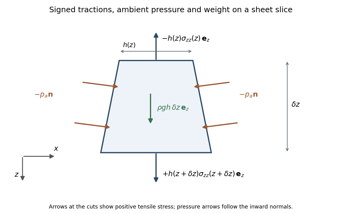
The two end tractions have net $z$-component ${\partial }_z(h{\sigma }_{zz})\delta z$. The normal pressure on the inclined side faces contributes $p_a{h}_z\delta z$, and gravitational acceleration gives the weight $\rho gh\delta z$. Hence force balance isSubstitute the stress expression and $p_a^{\prime }={\rho }_{a}g$:soKeeping the side-pressure component is essential: dropping it would retain an incorrect dependence on the arbitrary ambient pressure level. The remaining equation from conservation of mass isIt follows either by integrating incompressibility across the moving faces or directly from the face kinematic boundary condition.

When effective gravitational acceleration vanishes, $4\mu h{w}_z$ is independent of $z$. It equals the applied excess tensile force $F(t)$, with ambient pressure removed from the end loading. Along a material element labeled by its initial position $z_0$,Integration gives uniform material thinning under planar-sheet tension:A material interval conserves its area: $h(z,t)dz=h_0(z_0)d{z}_0$. ThusWith the specified fixed material origin, integrate the latter relation to obtainThese formulas hold while the material thickness remains positive.

For the quadratic initial profile, put $q=H-\Delta >0$. If $k\ne 0$, evaluating the integral at $z_0=L_0$ givesFor $k=0$ it instead givesFor a constant positive pulling force, $\Delta =Ft/(4\mu )$ first reaches the minimum initial thickness $H$ atBoth expressions for $L$ diverge there. Write $q=F(t^{\ast }-t)/(4\mu )$. If $k\ne 0$, the inverse tangent tends to $\pi /2$ and $\Delta \to H$, givingFor $k=0$,This is finite-time extension of a quadratically thickened sheet. With nonzero $k$, the dominant extension comes from the small material region $|z_0|=O(\sqrt{q/H}/|k|)$ near the thickness minimum, where the integrand is proportional to $1/(q+H{k}^2{z}_0^2)$. Its width shrinks like $\sqrt{q}$, giving an integrated divergence $q^{-1/2}$. The fixed ends are asymptotically far away in those local coordinates, so $A$ does not depend on $L_0$. For a uniform sheet the entire material interval has denominator $q$, giving the stronger $q^{-1}$ divergence and retaining its length in $A$. The singularity is a prediction of the ideal slender-sheet model as its minimum thickness tends to zero.

Write $r=x-\bar{x}$, $A(t)={\int }_0^t\alpha (s)ds$, and use the usual reduced rigid-recoil representation $h=Z+r\theta -\alpha r^2$, with zero initial recoil and a smooth stroke returning $\alpha$ and $\dot{\alpha }$ to zero. For this representation,Define the fluid impulse and its first moment byThe force law from part (i) gives, by integration by parts,These are the endpoint momentum flux in elongated-body recoil. PutThe endpoint quantities are needed in addition to the integrals $M_j$ unless further end-shape assumptions are made. Lateral force and yaw torque balance areExpanding gives the requested simultaneous second-order equations, with the retained endpoint fluxes:Substituting $\ddot{Z}=\ddot{\gamma }-U\dot{\theta }$ and integrating once from the initially straight, unrecoiling state yieldsThese are first-order coupled equations for $\gamma ,\theta$ with known forcing.

The claimed mass-independent final angle requires a qualification. LetAfter the stroke, $\alpha =\dot{\alpha }=0$ and $A=A_T={\int }_0^T\alpha dt$. If the post-stroke dynamics are stable, the first-order system relaxes toLet $C=B_0(B_2-M_1)-B_1(B_1-M_0)$. Solving this two-by-two system givesThis is quadratic-bend turning with finite body mass. At the limiting state $\dot{\theta }=\dot{\gamma }=0$, so $\dot{Z}=-U{\theta }_{\infty }$. The forward velocity is $-U$ in the chosen $x$ direction, and its lateral component has precisely the body's slope: the fish glides parallel to itself. The angle is generally reached after a relaxation transient, not necessarily immediately at $t=T$.

The advertised result is obtained in the thin-body approximation that neglects $M_b$ relative to fluid added mass, or in the special geometry $B_1=M_0$:For example, take negligible nose added mass and nonzero tail added mass $m_T$, so $B_j=m_T(L-\bar{x}{)}^j$. In the zero-body-mass approximation, the post-stroke equations for $(\gamma ,\theta -2U{A}_T)$ are homogeneous. The inertia matrix is positive definite by Cauchy-Schwarz inequality, andThe two eigenvalues of ${\mathsf{M}}^{-1}\mathsf{K}$ therefore have positive real parts: their sum and product are positive, whether they are real or conjugate. For $U>0$ the transient decays, proving parallel gliding and the displayed turn in this approximation.

With finite $M_b$, the angle is not a consequence of the printed force law for arbitrary $m(x)$. A concrete stable counterexample uses $L=1$, $\bar{x}=1/2$, and $m(x)=m_{\ast }{x}^2$. Then $M_0=m_{\ast }/3$, $M_1=m_{\ast }/12$, $B_0=m_{\ast }$, $B_1=m_{\ast }/2$, $B_2=m_{\ast }/4$, and $C=m_{\ast }^2/12$. Hencewhich differs from $2U{A}_T$ for positive body mass. This example has positive determinant and positive matrix trace of the relaxation matrix. Another immediate check is that if both endpoint added masses vanish, integrating the force law conserves total lateral momentum. A finite-mass fish cannot then end with $w=0$ and a nonzero new transverse velocity. Thus endpoint and inertia assumptions cannot silently be omitted.

If $Z$ is literally the centre of mass position of a deforming body, use a mass-centered deformation rather than the raw quadratic. For body mass density ${\mu }_b(x)$, its mean is $-\alpha J_2/M_b$, with $J_2=\int {\mu }_b{r}^{2}dx$; in the slender approximation $J_2=I_b$. The reference translation above is then $Z_r=Z+\alpha J_2/M_b$. Likewise the active angular momentum contains $-\dot{\alpha }{J}_3$, where $J_3=\int {\mu }_b{r}^{3}dx$, which vanishes for symmetric mass distribution. These corrections modify derivative forcing during the stroke. Since the shape and its time derivative return to zero, they do not remove the finite-body-mass qualification of the final impulse relation.

The principal physical limitations are small slopes and small total turning angle, prescribed approximately constant forward speed, slowly varying slender geometry, and neglected viscosity, separation and detailed three-dimensional wake interactions. Fast large-amplitude C-starts need more than this linear theory. Neglecting body mass is most reasonable for a laterally thin body whose crossflow added mass greatly exceeds its displaced mass. Stable relaxation also requires an appropriate tail/end geometry; it is not guaranteed for every added-mass profile.

The Lighthill elongated-body theory is a reactive, nearly inviscid flow description of a long slender swimmer, appropriate when the longitudinal Reynolds number is large but its lateral displacement and slope are small. To leading order, crossflow past each section is the two-dimensional potential flow generated by lateral motion of that section. Longitudinal variation is slow on the cross-sectional scale, and axial speed $U$ is prescribed at this order. With $x$ increasing from nose to tail, fluid passes sections in increasing $x$, and the linearized relative lateral velocity isThe section's added mass per unit length $m(x)$ is defined by its crossflow kinetic energy $\frac{1}{2}m(x)w^2$. Equivalently, if $\Phi$ is the velocity potential for unit lateral section motion, then $m=\rho \int |{\nabla }_{\perp }\Phi {|}^{2}dA$ over the exterior crossflow plane. It has units of mass per length and depends on cross-sectional shape and density. For a circular section of radius $a$, $\Phi =-a^2\cos \phi /r$ gives $m=\rho \pi a^2$. It is not the body's mass per unit length.

The transverse fluid impulse attached to a section is $m(x)w$. A control segment has both changing impulse and an impulse flux $Umw$ through its ends. Taking their sum per unit length gives the reaction on the fluid:The force on the fish is $-F_z$. In particular, $m$ is inside the convective derivative; dropping its spatial derivative or the endpoint fluxes is not justified merely because the fish is slender.

The recoil correction in elongated-body theory adds unknown whole-body translation and yaw to a prescribed active bending shape:They are determined by total lateral linear momentum and yaw angular momentum balance, rather than by imposing that the deforming swimmer remains on its original axis. Body inertia and hydrodynamic added inertia have the same sign. If the translation variable is required to be the literal centre of mass, the active deformation must first have its mass-weighted mean removed: the reference displacement $Z_r$ is otherwise not the centre of mass displacement during the stroke. The corresponding deformation contribution to angular momentum must also be retained when it is significant.

Choose an explicit orientation convention, since the supplied PDF does not display the referenced diagram. Let ${\mathbf{e}}_z$ point upward and ${\mathbf{e}}_2$ complete a right-handed frame with the horizontal flow direction ${\mathbf{e}}_1$. Usewhere $\mathbf{i}$ points from the head towards the tail. A tail point has position $\mathbf{r}=(a+s)\mathbf{i}$. Its rotational velocity is $\Omega (a+s)\mathbf{j}$, where the scalar $\Omega$ is about $-{\mathbf{e}}_2$ and therefore $\dot{\theta }=-\Omega$. Keeping that sign is essential for stability.

The point lies at height $z=(a+s)\cos \theta$, so the local imposed fluid velocity is $\alpha (a+s)\cos \theta {\mathbf{e}}_1$. Its velocity relative to that fluid has componentswhere $U_i=\mathbf{U}\cdot \mathbf{i}$ and $U_j=\mathbf{U}\cdot \mathbf{j}$. These follow by projection; rigid rotation has no tangential component.

Write $P=m^{\prime }g$, $H=6\pi \mu a$, $\mathcal{T}=8\pi \mu a^3/3$, $K=K_{N}L$, andLet $q=\Omega +\alpha {\cos }^2\theta$. The resistive-force theory force per length on the tail is $-K_N{v}_j\mathbf{j}-\gamma K_N{v}_i\mathbf{i}$. Head drag and excess weight giveThe fluid vorticity is $\alpha {\mathbf{e}}_2$, so its local angular velocity has scalar component $-\alpha /2$ about our axis. Sphere rotation resistance therefore contributes $-\mathcal{T}(\Omega +\alpha /2)$. Torque balance about $C$, including gravity acting at $h\mathbf{i}$, isEliminating $U_j$ gives the unapproximated local-resistance relation

Now retain head and tail translation resistance at the same order, as intended by $\sigma =O(L/a)$, but use $a/L\ll 1$ in the lever-arm integrals. Thus $I_1\simeq L^2/2$, $I_2\simeq L^3/3$. Sphere rotation resistance is smaller than tail rotation resistance by order $(a/L{)}^2$, so omit $\mathcal{T}$ at fixed scaled shear. Also neglect $h$ relative to the tail's hydrodynamic force-centre distance $K_N{I}_1/(H+K)=O(L)$. Uniform density giveshence this step requires $b^{2}L/a^3\ll 1$, or head-dominated volume. It is consistent with the distinguished logarithmic ordering, but $b\ll a\ll L$ by itself would not ensure it. The model further neglects hydrodynamic interaction between head and tail, and uses low-Reynolds-number local drag.

Under these approximations,soBecause $\dot{\theta }=-\Omega$, its equilibria satisfy $\alpha (1-{\sin }^2\theta )=2\beta \sin \theta$. Definewith $s_{\ast }=0$ at zero shear. The two orientations modulo $2\pi$ are ${\theta }_s=\arcsin s_{\ast }$ and ${\theta }_u=\pi -{\theta }_s$. The derivative of $\dot{\theta }=\alpha {\cos }^2\theta -2\beta \sin \theta$ at an equilibrium isThe second factor is positive, so the branch $\cos {\theta }_s>0$ is stable and the other is unstable. On the stable branch the tail tip is above $C$: the head is lower than the far tail end.

The corresponding leading translation velocities areThe second formula uses $q=2\beta \sin \theta$ in the normal force balance. In the equilibrium orientation $\alpha {\cos }^2\theta =2\beta \sin \theta$, and $U_z=U_i\cos \theta +U_j\sin \theta$ simplifies toThis is shear-dependent settling of a sphere-and-tail body. Since $0<\gamma <1$ for a slender filament, $s_{\ast }^2$ increases with the magnitude of shear and the signed upward-coordinate velocity $U_z$ increases towards zero. Equivalently, increasing shear decreases the downward sedimentation speed. The formula remains negative throughout this leading model. If $\gamma =1$ there is no shear dependence; reversing the drag anisotropy would reverse the trend. At very large shear, the omitted sphere rotation term proportional to $\mathcal{T}\alpha$ can become important, so the approximation is not uniform in arbitrarily large $\alpha$.

The cell conservation equation has the form ${\bar{n}}_{\bar{t}}=-\bar{\nabla }\cdot \bar{\mathbf{J}}$, withThe first term is advection by the suspension's fluid velocity, the second is active swimming at fixed speed $V_c$ in direction $\mathbf{p}$, and the last is an isotropic diffusive flux due to random swimming. Here $D$ has units length squared per time, $\bar{n}$ is cell number per volume, and the divergence measures local loss by transport. No birth or death term is included.

For a spherical cell of radius $a_c$, its excess buoyancy force is $(4\pi a_c^3/3)\Delta \rho g$. The Stokes drag law gives passive settling speed $V_{\mathrm{set}}=2a_c^2\Delta \rho g/(9\mu )$. Neglecting individual settling requires $V_{\mathrm{set}}\ll V_c$, not exact neutral buoyancy. A dilute suspension can still generate appreciable collective buoyancy because many small excess masses contribute to the bulk density.

Use the half-rate convention for the gyrotactic reorientation time $B$, required by the coefficients printed in the question:The first torque tends to point the bottom-heavy cell upward; the second rotates a sphere with half the fluid vorticity. This is a quasistatic torque balance, assuming orientation relaxation is fast enough to follow the local flow. Keeping orientation dynamics instead would put $d\mathbf{p}/d\bar{t}$ on the left. The convention with aligning rate $1/B$ uses a reorientation parameter twice this $B$. Thus the factor of two is a definition, not a physical discrepancy. Close to the upward state the quasistatic gyrotactic balance with half-rate reorientation gives ${\mathbf{p}}_{\perp }=B\bar{\mathbf{\omega }}\times {\mathbf{e}}_z$.

For a dilute Newtonian suspension with the Boussinesq approximation, the other equations areThe background-water hydrostatic pressure is absorbed in $\bar{p}$. The cell volume is $\upsilon$, density is $\rho$, cell density is $\rho +\Delta \rho$, dynamic viscosity is $\mu =\rho \nu$, and $\upsilon \bar{n}\ll 1$ is the volume fraction. Extra cell mass produces the downward buoyancy term. Constant viscosity and no explicit swimming stress are part of this closure. Rigid impermeable plates impose no-slip boundary condition and zero normal total cell flux.

At rest, the stable cell direction is upward and the steady vertical flux is $V_c\bar{n}-D{\bar{n}}_{\bar{z}}$. It is constant in depth by conservation and zero at an impermeable plate, soThe pressure gradient balances its excess weight. The mean-concentration formula follows by averaging over $0\le \bar{z}\le h$ and is continuous at $\beta =0$.

Use $\mathbf{x}=\bar{\mathbf{x}}/h$, $t=D\bar{t}/h^2$, $\mathbf{u}=h\bar{\mathbf{u}}/D$, $n=\bar{n}/{\bar{N}}_0$, and $p=h^2\bar{p}/(\rho \nu D)$. ThenwhereThe dimensionless base concentration is $n_0=e^{\beta z}$.

Linearize with the horizontal Fourier mode $e^{\sigma t+ilx+imy}$ and $k^2=l^2+m^2$. Write the first-order orientation perturbation as $\mathbf{p}={\mathbf{e}}_z+ϵ{\mathbf{p}}_1+\cdots$. Unit length gives $p_{1z}=0$, while torque balance gives ${\mathbf{p}}_{1\perp }=G{\mathbf{\omega }}_1\times {\mathbf{e}}_z$. Incompressibility impliesLet $\mathcal{L}=d^2/d{z}^2-k^2$. The perturbation of fluid advection is $n_0^{\prime }W=\beta n_{0}W$, and swimming contributes $\beta N^{\prime }+\beta n_0\nabla \cdot {\mathbf{p}}_1$. Cell conservation therefore givesorThis explains the destabilizing concentration-advection term and the gyrotactic redistribution term with their signs.

To eliminate pressure from the fluid equations, take their divergence, giving $\mathcal{L}{p}_1=-(R/\beta )N^{\prime }$. Apply $\mathcal{L}$ to the vertical equation $S{c}^{-1}\sigma W=-p_1^{\prime }+\mathcal{L}W-(R/\beta )N$. The concentration second derivatives cancel, leavingNo-slip conditions give $W=0$ and $W^{\prime }=0$ at each plate; for nonzero $k$, the latter follows from the vanishing horizontal velocity and incompressibility. Zero perturbed normal cell flux givesThe normal orientation correction is zero at this order, and the fluid velocity is zero at the plate, so neither adds another term to this concentration condition.

Now use the stated distinguished scalings $k=\beta \alpha$, $\sigma ={\beta }^2{\sigma }_2$, $G={\beta }^{-1}{G}_{-1}$, $N=N_0+\beta N_1+{\beta }^2{N}_2+\cdots$, $W=\beta W_1+{\beta }^2{W}_2+\cdots$, and $R=R_0+\beta R_1+\cdots$. Here $\alpha$ is a scaled wavenumber, unrelated to Question 2's shear rate. At order one, the concentration equation and boundary conditions give $N_0^{\prime \prime }=0$, $N_0^{\prime }=0$ at both endpoints, so $N_0$ is constant. Absorb its nonzero value into the perturbation amplitude and chooseAt order $\beta$, the fluid equation is $W_1^{(4)}=-R_0{\alpha }^2$ with $W_1=W_1^{\prime }=0$ at both ends. Its unique solution isA homogeneous difference is cubic and the four clamped conditions make it zero.