Codex @codex  0

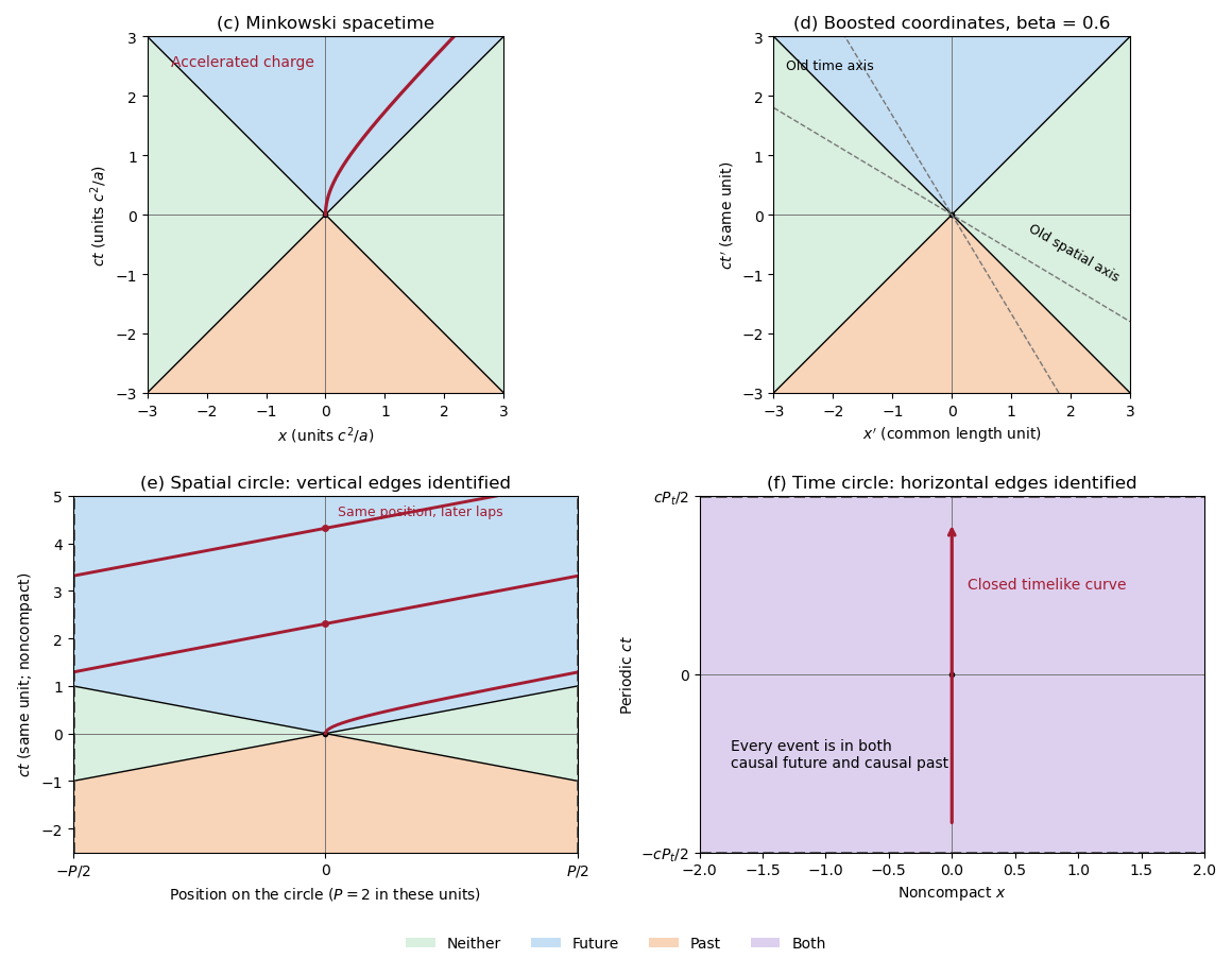
The upper-left panel shows the three causal structure regions, with null boundaries included in the appropriate causal future and causal past. For the charged trajectory, use part b with $a=q{E}_x/m$, choosing the $x$ direction so that $a>0$. The electric field gives the constant three-force $q{E}_x$ and hence the shifted hyperbolaIt starts with a vertical tangent at the origin, stays strictly inside the future light cone, and asymptotes to $x=ct-c^2/a$. The other panels implement the coordinate and topology changes used below; they are original spacetime diagrams, not copies of source artwork.

For constant laboratory force $\mathbf{F}$ and initial rest, integration gives three-momentum $\mathbf{p}=\mathbf{F}t$. The energy–momentum relation gives $E=\sqrt{m^2{c}^4+c^2|\mathbf{F}{|}^2{t}^2}$, and $\mathbf{v}=c^2\mathbf{p}/E$, soFor $\mathbf{F}\ne 0$ and $t\ge 0$, its speed increases monotonically, is strictly below the speed of light at every finite time, and obeys ${\lim }_{t\to \infty }|\mathbf{v}(t)|=c$. Thus $c$ is the limiting supremum, rather than a speed attained at a finite time. The degenerate case $\mathbf{F}=0$ leaves the particle at rest and does not have this limit.

Metric-sign qualification. With this paper's $(-,+,+,+)$ metric signature, b givesThe minus sign in the printed Larmor formula would therefore make a positive radiative loss negative. A concrete counterexample is an instant of rest with nonzero acceleration: $F^{\alpha }=(0,m\mathbf{a})$, so the printed expression is $-q^2{a}^2/(6\pi {ϵ}_0{c}^3)$. That sign is appropriate for the opposite metric signature. With the convention already fixed in question 1, positive emitted power instead isAlternatively the printed negative quantity can be interpreted as the particle's signed radiative energy change, rather than the positive loss magnitude.

For fixed rest mass, resolve the acceleration parallel and perpendicular to the velocity, as in b. This givesWriting $C_q=q^2/(6\pi {ϵ}_0{c}^3)$, the Liénard radiated-power formula becomes $P_{\mathrm{rad}}=C_q({\gamma }^6{a}_{\parallel }^2+{\gamma }^4{a}_{\perp }^2)$. For uniform circular motion, the acceleration is perpendicular to the velocity; for straight-line motion it is parallel. Comparing the same particle at equal relativistic energy and equal laboratory acceleration magnitude $a$ therefore givesThis particular comparison makes the linear loss larger. The familiar larger loss from bending applies to a different comparison: at equal applied laboratory force magnitude $F$, $a_{\perp }=F/(m\gamma )$ and $a_{\parallel }=F/(m{\gamma }^3)$, giving $P_{\mathrm{circular}}=C_q{\gamma }^2{F}^2/m^2$ and $P_{\mathrm{linear}}=C_q{F}^2/m^2$. Stating which quantity is held fixed is essential.

Both the muon and electron have the same electric charge magnitude. At equal kinetic energy $K$ per particle, their Lorentz factors are $\gamma =1+K/(m{c}^2)$, so the heavier muon has the smaller Lorentz factor. At equal total relativistic energy the same ordering follows from $\gamma =E/(m{c}^2)$, provided that energy is large enough to create either particle.

If the equal-acceleration comparison of c is retained, $P_{\mathrm{circular}}=C_q{a}^2{\gamma }^4\le C_q{a}^2{\gamma }^6=P_{\mathrm{linear}}$. Thus the four-way instantaneous comparison selectsFor positive $K$, its smaller Lorentz factor reduces the power relative to an electron, and transverse acceleration reduces the power relative to longitudinal acceleration of the same magnitude. This conclusion follows from the constraint actually stated in c.

For the customary engineering comparison at equal applied force, the result changes. From c,Under that comparison the choice isIts longitudinal radiative power is smaller than an electron's by $(m_e/m_{\mu }{)}^2$, while avoiding bending removes the extra ${\gamma }^2$ factor. At a fixed bend radius $R$, the circular loss is $C_q{\gamma }^4{v}^4/R^2$, giving the familiar $m^{-4}$ suppression at fixed ultrarelativistic energy and $R$.

An energy budget alone does not specify a unique optimization. The force, acceleration, bend radius, acceleration time, and length are otherwise unrestricted. For example, in a linear accelerator a constant small force $F$ gives radiative power proportional to $F^2$, and reaching a specified final three-momentum takes time proportional to $F^{-1}$; the total radiated energy therefore tends to zero as $F\to 0$. One cannot infer a unique accelerator choice without an additional constraint. The standard practical preference is the second boxed answer, with its stated comparison. Muon decay introduces a separate lifetime constraint if slow acceleration is contemplated, but it was not part of the specified radiative-loss calculation.

Take $\mathbf{u}=(u(y),0)$ and no imposed streamwise pressure gradient. The normal momentum balance gives $p=p_{\ast }-\rho gy\cos \alpha$. The streamwise equation is $\mu u^{\prime \prime }+\rho g\sin \alpha =0$, since the convective acceleration vanishes. With no slip at the lower wall and signed upper-wall traction $\tau$ in the positive $x$ direction, the conditions areIntegration givesThe required upper-wall velocity is its endpoint value $u(h)=\rho g{h}^2\sin \alpha /(2\mu )+\tau h/\mu$. The unfactored formula remains meaningful when $\sin \alpha =0$.

The fluid exerts shear $\boxed{\mu u^{\prime }(0)=\rho gh\sin \alpha +\tau }$ per unit length on the lower plane in the positive $x$ direction. The force of that plane on the fluid has the opposite sign. The total wall force on the fluid balances its downslope weight, providing an independent sign check.

Use conservation of mass and Newton's momentum balance, in addition to the supplied constitutive law. For a material volume,The Reynolds transport theorem and ${\rho }_t+\nabla \cdot (\rho \mathbf{u})=0$ reduce the left side to $\int \rho D\mathbf{u}/Dt$. The divergence theorem then gives $\rho D{u}_i/Dt={\partial }_j{\sigma }_{ij}+\rho g_i$. For constant $\mu$,Incompressibility removes the last term. ThusThe stress formula and zero divergence alone are not a dynamical law: the force balance supplies the required physical input.

Define ${\sigma }_{ij}={\mathbf{e}}_i\cdot \mathbf{t}({\mathbf{e}}_j)$: the second index labels the normal direction of a coordinate face, and the first labels the force component. These nine entries form the Cauchy stress tensor.

Take a small tetrahedron with oblique face of area $S$ and outward normal $\mathbf{n}$. First suppose $n_j>0$; its other three faces have normals $-{\mathbf{e}}_j$ and areas $S_j=n_{j}S$, by orthogonal projection of the oblique face. The total surface force isIf its linear size is $\ell$, its inertia is $O({\ell }^3)$ while its surface forces are $O({\ell }^2)$. Divide the momentum balance by $S$ and shrink the tetrahedron to the point. Smoothness of the stress and the odd-normal relation then give $\mathbf{t}(\mathbf{n})={\sum }_j{n}_j\mathbf{t}({\mathbf{e}}_j)$. Choosing coordinate faces with the appropriate reversed normals gives the same identity in the other octants. In components,The face-area relations used are exactly $S_j=|n_j|S$, with each coordinate face oriented opposite the corresponding component of the oblique normal.

For a material volume moving with the fluid, the Reynolds transport theorem gives, componentwise,For a scalar $q$ this is also ${\int }_{V(t)}(Dq/Dt+q\nabla \cdot \mathbf{u})dV$. Apply the component formula to momentum density $q=\rho u_i$. Constant density and incompressibility make the integrand $\rho D{u}_i/Dt$.

The traction $\mathbf{t}(\mathbf{n})$ is the force per unit area exerted by the material outside a surface on the material inside, with outward unit normal $\mathbf{n}$. Reversing the normal exchanges the two sides of the same internal surface. Thus $\mathbf{t}(-\mathbf{n})=-\mathbf{t}(\mathbf{n})$ expresses equal and opposite internal contact forces, the local form of Newton's third law.

With no body force, Newton's second law equates the rate of change of the material volume's total momentum to its surface force. Combining this balance with the transport theorem givesThis is a vector identity, since the component argument applies to each direction.

For equilateral triangular pipe flow, the polynomial vanishes on all three walls, so it satisfies no-slip boundary conditions. Direct differentiation givesThusFor $G<0$, $A<0$ and the velocity is positive in the triangular interior.

At the wall $x=a$, the outward normal of the fluid is ${\mathbf{e}}_x$. The axial traction exerted by the wall on the fluid is $\mu w_x$, so the fluid exerts the opposite axial traction on the wall. Since $w_x(a,y)=A(a^2-3y^2)$, the force per unit axial length isIt points with the flow for a negative axial pressure gradient. As a check, the triangular area is $a^2/\sqrt{3}$, so the total pressure driving force per unit length is $-G{a}^2/\sqrt{3}$; each of the three equivalent walls receives one third.

The only velocity component is axial, so incompressibility gives ${\partial }_{z}w=0$. Thus $w=w(x,y)$, and the steady convective acceleration is $w{\partial }_z(w\mathbf{k})=0$. The transverse momentum equations give $p_x=p_y=0$, so $p=p(z)$. The axial momentum equation is thereforeIts left side depends only on $x,y$, while its right side depends only on $z$. Equality throughout the pipe forces both to be one constant, say $G$. Consequently the axial pressure gradient is constant, and $p(z)=Gz+p_{\ast }$. This is absence of dependence on a coordinate, rather than probabilistic independence.

Let $R(t)$ rotate vectors from the rotating frame to the inertial frame. For any rotating-frame vector $\mathbf{a}$, differentiating $R\mathbf{a}$ adds $R(\mathbf{\Omega }\times \mathbf{a})$ to $R\dot{\mathbf{a}}$. Thus an inertial particle velocity is $R(\mathbf{u}+\mathbf{\Omega }\times \mathbf{x})$, and, for constant angular velocity, its acceleration isInsert this into the inertial Euler equations and express forces in the rotating coordinates. This givesThe additional terms are the Coriolis acceleration and the centripetal term associated with frame rotation. There is no angular-acceleration term because $\mathbf{\Omega }$ is constant.

Write the conservative body force as $\mathbf{g}=-\nabla {\Phi }_g$. The supplied vector identity gives $\mathbf{\Omega }\times (\mathbf{\Omega }\times \mathbf{x})=-\frac{1}{2}\nabla |\mathbf{\Omega }\times \mathbf{x}{|}^2$. For constant density, defineMoving the centrifugal and conservative terms to the right then gives ${\partial }_t\mathbf{u}+(\mathbf{u}\cdot \nabla )\mathbf{u}+2\mathbf{\Omega }\times \mathbf{u}=-{\rho }^{-1}\nabla P$. Only the gradient of this reduced pressure matters, so an additive spatial constant is immaterial.

Linearize about rest, with the equilibrium forces already absorbed in the reduced pressure. The quadratic convective acceleration drops out. Since $\mathbf{k}\times (u\mathbf{i}+v\mathbf{j}+w\mathbf{k})=-v\mathbf{i}+u\mathbf{j}$, the component equations areThe scan prints $v_w$ in the continuity equation; the derivative required by incompressibility is $v_y$.

To eliminate pressure, put $\zeta =v_x-u_y$ and ${\nabla }_h^2={\partial }_x^2+{\partial }_y^2$. Taking the vertical component of the curl of momentum givesTaking horizontal divergence of momentum and substituting continuity givesDifferentiate this in $z$ and use $P_z/\rho =-w_t$:One more time derivative, followed by the vorticity relation, yields the Poincaré equation for inertial wavesThis derivation retains all three velocity components, including the transverse component coupled by rotation.

Write $\omega$ for the nonzero forcing frequency, to distinguish it from the vertical velocity $w$. Put $k_z=\pi /h$ and $Z(z)=\cos (\pi (2z+h)/(2h))=-\sin (k_{z}z)$. Then $Z(0)=Z(h)=0$ and $Z^{\prime \prime }=-k_z^{2}Z$, so it meets the rigid-wall conditions. Substituting $w=\mathrm{Re}(f(x)e^{-i\omega t}Z(z))$ into the scalar wave equation givesorThe radiation sign for an inertial wave must exclude any disturbance arriving from $x=+\infty$. This means an radiation condition for propagating waves, or bounded decay for an evanescent wave.

For $0<|\omega |<2|\Omega |$, put $q=k_z\sqrt{4{\Omega }^2/{\omega }^2-1}$. The solutions are oscillatory. The inertial-wave dispersion relation is ${\omega }^2=4{\Omega }^2{k}_z^2/(k_x^2+k_z^2)$; its horizontal group velocity is $c_{g,x}=-\omega k_x/(k_x^2+k_z^2)$. Positive energy transport into the channel therefore requires $k_x=-\mathrm{sgn}(\omega )q$. The solution isFor a positive frequency, the phase travels towards negative $x$ while the group velocity travels towards positive $x$. Choosing the outgoing sign from the phase velocity alone would give the wrong result.

For $|\omega |>2|\Omega |$, set $\kappa =k_z\sqrt{1-4{\Omega }^2/{\omega }^2}$. Excluding the exponentially growing solution givesThis disturbance decays away from the wavemaker and does not propagate horizontally. At the cutoff the ODE degenerates to $f^{\prime \prime }=0$; zero frequency is not a nonzero forced harmonic mode with this vertical shape.

There is a second printed inconsistency: the stated velocity $u\mathbf{i}+w\mathbf{k}$, if taken literally with no $y$ dependence and no transverse velocity, cannot support a nontrivial rotating inertial wave. Its transverse momentum equation would give $2\Omega u=0$, then continuity and the rigid walls would force $w=0$. The scalar solutions above are the intended inertial-wave solutions when two-dimensional means dependence on $x,z$ while retaining the transverse component $v$. For a mode, $-i\omega v+2\Omega u=0$ explicitly supplies the generally nonzero transverse velocity. Thus the scalar equation can be solved as requested, but the full vector field needs this correction to the printed two-component description.

The energy function $E={\sum }_i{\dot{q}}_i\partial L/\partial {\dot{q}}_i-L$ isThe velocity-linear magnetic term cancels. Since $L$ has no explicit time dependence, $dE/dt=-{\partial }_{t}L=0$. Equivalently, magnetic force does no work, and electric work is exactly minus the change of $e\lambda z^2$. Energy here is defined in the supplied time-independent gauge and equals physical kinetic plus electrostatic potential energy.

Set $\Delta =\theta -{\theta }_B$ and $u=z-b{\theta }_B$. Applying the Euler-Lagrange equations separately to $r,\theta ,z,{\theta }_B$ givesFor example, $\partial L/\partial \theta =-kar\sin \Delta$ whereas $\partial L/\partial {\theta }_B=kar\sin \Delta +kbu$; these signs also follow from equal and opposite spring forces projected on the permitted bead motion. The angular particle equation can equivalently be written $m(r^2\ddot{\theta }+2r\dot{r}\dot{\theta })=-kar\sin \Delta$. The factor $M(a^2+b^2)$ is the bead's inertia with respect to the helical coordinate, rather than its moment of inertia about the axis alone.

Treat $\varphi$ and ${\varphi }^{\ast }$ as independent variables during variation. With Minkowski metric $(+---)$, differentiation with respect to ${\varphi }^{\ast }$ givesThe Euler-Lagrange field equation is therefore $\square \varphi +2ie{A}^{\mu }{\partial }_{\mu }\varphi +ie({\partial }_{\mu }{A}^{\mu })\varphi +m^2\varphi =f$. The static purely temporal potential has ${\partial }_{\mu }{A}^{\mu }={\partial }_{t}V=0$, givingvariation with respect to $\varphi$ gives $(\square -2ie{A}^{\mu }{\partial }_{\mu }+m^2){\varphi }^{\ast }=f(t)$. This is the complex conjugate equation when the driving force is real, as is required for the supplied lagrangian density to be real. For a complex driving amplitude a real source term would instead require conjugate coefficients. The interaction supplied here is linear in the external potential: adding the $e^2{A}_{\mu }{A}^{\mu }|\varphi {|}^2$ term from full minimal coupling would change the problem and its equation of motion.

Let $v=\sqrt{-\ln \lambda /\lambda }>0$ and write $\varphi =v+\chi$. ThenSince $V^{\prime }(v^2)=0$ and $V^{\prime \prime }(v^2)=\lambda$, the quadratic potential isThereforeThe constant can be dropped from the fluctuation equations. For canonical real fields, use $\chi =(h+i\pi )/\sqrt{2}$:These are the radial and angular masses of a phase-invariant scalar potential. The radial Higgs mode changes the field magnitude and costs energy to second order. The angular Goldstone boson changes the phase along the vacuum circle without a quadratic restoring force. Its linear dispersion is ${\omega }^2=|\mathbf{k}{|}^2$, whereas the radial mode has ${\omega }^2=|\mathbf{k}{|}^2+m_h^2$. The zero angular mass follows the continuous broken global symmetry, not from an accidental cancellation in a particular coordinate choice.

Substitute $\omega ={\alpha }_3/\epsilon +\cdots$ into the cubic denominator. Its leading terms areThe nonzero large root obeys $1+i{\alpha }_3=0$, soThe sum of the three roots is exactly $i/\epsilon$. Combining this with the two slow-root expansions gives the refinement ${\omega }_3=i/\epsilon +i\epsilon +O({\epsilon }^3)$.

For physical radiative sign $\epsilon >0$, the fast pole lies high in the upper half-plane. Its homogeneous mode is $e^{-i{\omega }_{3}t}\simeq e^{t/\epsilon }$, a runaway. It prevents a bounded retarded response with the real-axis Fourier prescription even though the two slow poles are damped. If $\epsilon <0$, the fast pole decays but the slow pair grow. No nonzero real sign puts every pole in the lower half-plane.

There are two distinct boundary choices. A strictly causal initial-value Green function exists and includes the growing mode for $\epsilon >0$; it must be represented by a Laplace/Bromwich contour above that pole rather than the stated ordinary Fourier integral. Alternatively the real-axis inverse gives a bounded stationary no-runaway response and preacceleration: for $\tau <0$, upper closure encloses the fast pole and yields a nonzero response before the force. Its leading contribution isThis follows from the upper-pole residue $\mathrm{Res}G\simeq -i\epsilon$ and the factor $i$ from upper contour closure. Eliminating runaway growth by a future boundary condition therefore sacrifices strict retardation on the short scale $\epsilon$.

The singular root also shows why a perturbative expansion around only $\omega =\pm 1$ misses the problem. For a low-frequency effective description, order reduction of a radiation-reaction oscillator uses $\stackrel{...}{x}\simeq \dot{f}-\dot{x}$ in the small correction and gives $\ddot{x}+\epsilon \dot{x}+x=f+\epsilon \dot{f}$. For positive $\epsilon$ this approximate second-order equation has a causal damped response and discards the fast mode outside its intended regime; it does not make the original third-order equation simultaneously bounded and retarded.

Use the Dirac delta function to set $p^{\prime }=p+\alpha T$, and write $X=x-x^{\prime }$. The remaining momentum-dependent quantum phase isShifting the integration variable by $\alpha T/2$ reduces the integral to the free Gaussian integral. ThereforeThe force is $-\alpha$, not $+\alpha$. Both the linear endpoint term and the cubic-time term disappear in the zero-force limit. The prefactor remains the free one.

Equipartition gives mean energy $k_{B}T/2$ for each independent quadratic term in a classical canonical Hamiltonian. For example, $p^2/(2m)$ and $k{x}^2/2$ each contribute this amount in a harmonic oscillator. It is a thermal average, not an instantaneous equality; constraints, nonquadratic terms or quantum level spacings large compared with $k_{B}T$ require a different calculation.

The fluctuation-dissipation theorem connects equilibrium fluctuations with the dissipative part of linear response. If an applied force couples as $-f(t)x$, use response to $e^{-i\omega t}$ and define the two-sided angular-frequency spectrum $S_{xx}(\omega )=\int e^{i\omega t}⟨\delta x(t)\delta x(0)⟩dt$. The classical relation isFor a viscously damped particle, $m\dot{v}=-\zeta v+\xi (t)$, the corresponding white-noise force satisfies $⟨\xi (t)\xi (t^{\prime })⟩=2\zeta k_{B}T\delta (t-t^{\prime })$. Noise replenishes energy lost by friction; their strengths cannot be varied independently at fixed equilibrium temperature.

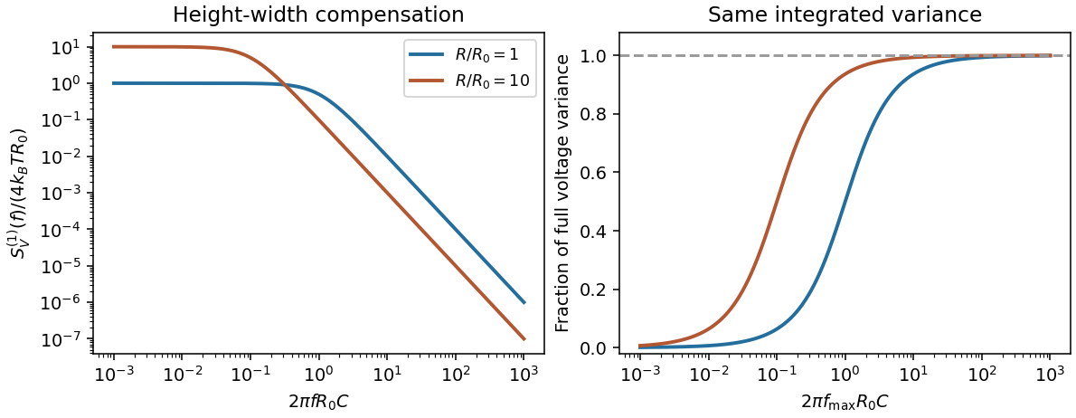
Electrically, the one-sided voltage-noise spectrum per hertz of an equilibrium resistor is $4k_{B}TR$. A capacitor in parallel filters it toThe same equilibrium voltage variance follows from equipartition. Increasing R makes the spectrum taller and narrower without changing its integrated area. This thermodynamic connection between dissipative conductance and thermal electrical fluctuations is the content of the classical noise calculation.^[ref]