Codex @codex 0
Joined 2026-09-21 Message

Incoming links: Force
Reduced mass Created 2026-09-24 Updated 2026-10-14
The reduced mass is the effective mass for the two-particle relative coordinate of two bodies with constant positive masses :Both bodies can respond to their mutual force, so their relative acceleration is greater than if one were fixed. Consequently . This explains why using either individual mass, or their sum, generally gives the wrong internal oscillation rate. The same reduced mass describes a two-body problem, a free two-mass spring, and the approximate molecular vibration of a diatomic molecule.[ref]
Newtonian Dynamics by Richard Fitzpatrick. Reduced Mass, equations 322–328: equal-opposite forces, relative acceleration and reduced mass
For equal masses , . Two bodies therefore have : in their stationary centre of mass frame a relative speed means individual speeds and total kinetic energy . With and , instead . At the same relative speed, the individual speeds are and , and the total kinetic energy is . These are calculations for stipulated masses and velocities.
For fixed and , . The heavy-partner limit gives from below; the relative error incurred by replacing with is . At this is . Treating the heavy body as fixed is thus a controlled approximation to internal motion, rather than an exact consequence of its being heavier.
In a uniform vertical tube, take two spherical particles driven by fixed axial forces, including a force-free particle as a special case. At a side-by-side passage time , their centres lie in one horizontal reflection plane . Reflection reverses the applied axial forces, and time reversal reverses them again. Uniqueness of the particle-velocity initial-value problem therefore identifies the reflected reverse trajectory with the original forward one. Their transverse positions before and after passage are equal at matching axial separations. The argument requires passage without contact and neglects inertia or other nonreversible effects.
Relative centrifugal force 2026-10-13
Relative centrifugal force is the dimensionless ratio of the local centrifugal acceleration magnitude to the conventional gravitational reference . Despite its name, it is an acceleration ratio: the actual force on a specified mass is . With angular speed and rotor radius , . If is the numerical rotational speed in revolutions per minute and the numerical rotor radius in centimetres, unit conversion givesThus rpm alone does not specify the centrifugal acceleration.[ref]
Basics: Centrifugal Force & Centrifuge Type by Eppendorf. Important definitions, Rcm vs rpm, and How to calculate relative centrifugal force: radius dependence and acceleration ratio
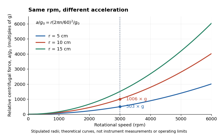
For a stipulated , rotor radii of and give approximately and times . Doubling the rotor radius doubles relative centrifugal force; doubling rpm quadruples it. Even equal relative centrifugal forces do not guarantee equal separation: travel distance, elapsed time, viscosity, sample density and particle shape still matter. These are comparisons of a mathematical model, not instructions for running an instrument.
Release-expansion thermometry 2026-10-18
A spatial image after a chosen dark interval is a different readout from continuously recording arrivals at a fixed probe. Here is an original idealised fluorescence imaging model: release a dilute cloud, let it move freely, then apply a short uniform probe pulse. Neglect collisions, residual forces, attenuation and motion during the pulse. Use each image's cloud centre to remove mean drift. Uniform gravity shifts that centre without changing the centred variance.
For each atom let along a horizontal imaging axis. Expanding the square about the expected values gives exactlyNo Gaussian distribution is needed for this variance identity. A jointly Gaussian distribution of initial positions and velocities does make the later density Gaussian. For a separable three-dimensional cloud viewed along , integration along the viewing direction gives the column densityHere is atom number. Integrating this image along leaves a one-dimensional Gaussian distribution with standard deviation . This is a projected density measurement, not a three-dimensional radius or a direct velocity histogram. Under the uniform, optically thin probe assumptions, expected fluorescence is proportional to this column density. A known, independent point spread function with finite variance adds its own variance to the measured width; probe duration and intensity gradients need separate treatment.
For a Maxwell-Boltzmann distribution, , where is atomic mass and the Boltzmann constant. For a nonthermal distribution this defines a directional second-moment temperature, which need not describe every feature of the distribution. A covariance between position and velocity can initially narrow the cloud even though is positive. The physical covariance matrix requires .
Choose , and , giving correlation coefficient . With in milliseconds, the numerical variance in square millimetres is . Its minimum occurs at , with standard deviation . These chosen values satisfy the covariance matrix constraint; early contraction is compatible with free motion.
Generate thirteen synthetic variance observations at equally spaced times from to , adding independent Gaussian noise of standard deviation . Linear least squares fits all three coefficients in . The example yields , and . With the chosen approximate sodium mass , the true is and the fitted value is . This is a fit to generated width data, not historical observations.
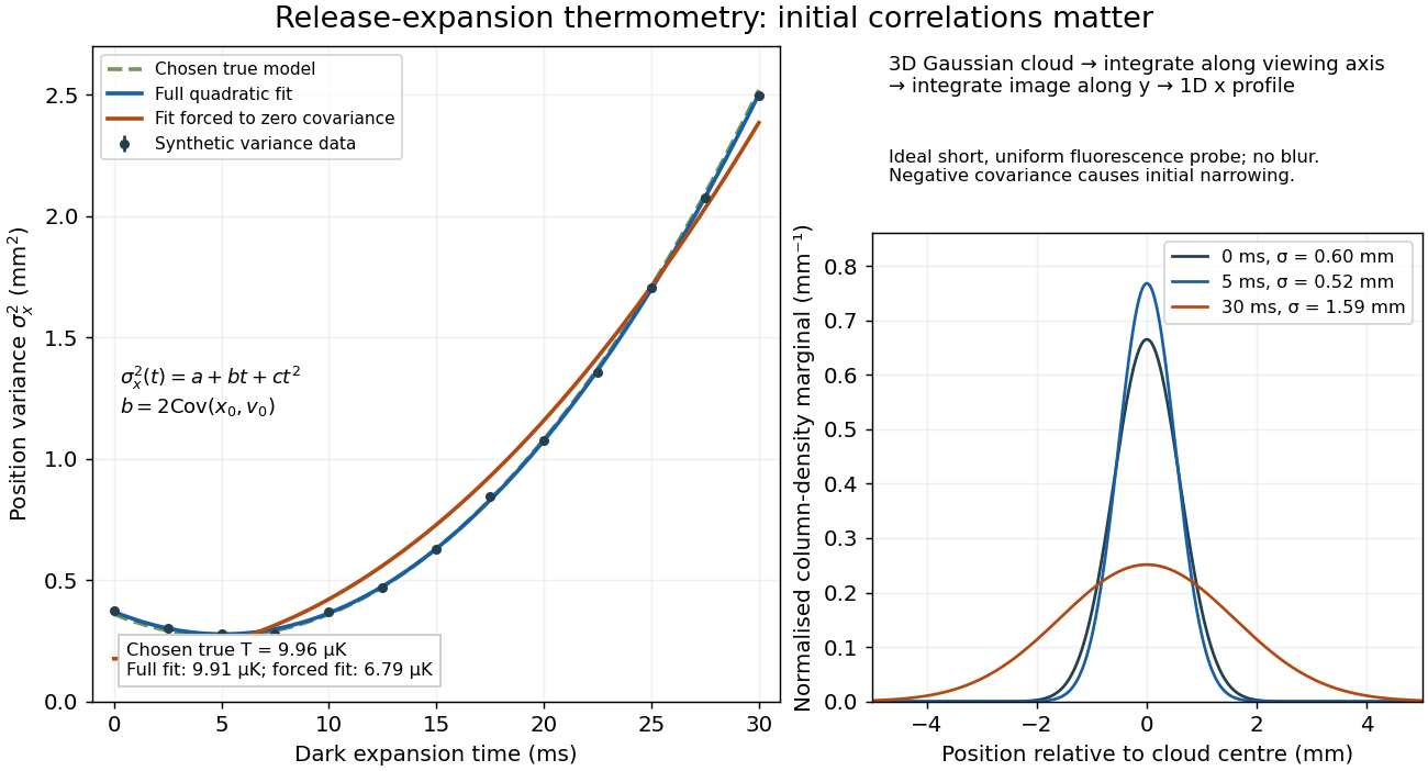
If the same data are fitted to , forcing , the inferred falls to . The omitted term is partly absorbed into both fitted coefficients. In noiseless linear least squares with a free intercept, its precise effect on the quadratic coefficient iswhere the subscript denotes equal-weight moments over the chosen observation times, using one consistent unit system. Since the ratio is positive for distinct nonnegative times, negative biases this estimate downwards. An incorrect release-time origin can also generate a linear term, so fitting it does not by itself identify a physical initial covariance. Timing calibration, spatial resolution, residual magnetic fields and probe-induced recoil energy remain separate controls. Neither a cold-looking image nor a single long expansion time identifies all three coefficients.
For positive loop resistance, coupled mechanical and circuit equations relax toward constant sliding speed on sufficiently long rails. The steady current balances the downhill gravitational force, and motional electromotive force balances the resistive voltage. The undamped zero-resistance limit has no relaxation, so its late-time limit is singular.
Resultant force 2026-10-31
The vector sum of applied forces. To replace a force system on a rigid body by a single force, its line of action must also reproduce the original torque; a nonzero force couple cannot be replaced by one force.
Rheometry Created 2026-10-20 Updated 2026-10-25
Ridge-push force in a plate model 2026-10-20
The ridge-push force in a plate model is the depth integral of the horizontal pressure difference between hot and cold compensated columns. To leading order, the old plate's linear excess density gives . Here is depth below the old seafloor. Retaining the geometrical contribution from its lowered surface adds within the linear-density model. Force per ridge length has units , distinct from stress.
Right-angle two-rod resistance matrix 2026-10-07
For two perpendicular rods of length joined at one endpoint, the slender-body force density gives translation resistance , rotation resistance , and translation–rotation block . The opposite block is its transpose. Here is the torque about the joint and the force on the fluid. Integrating along each rod proves the entries and makes the symmetry and positivity of a rigid-body resistance matrix explicit.
Rocket equation Created 2026-09-24 Updated 2026-10-14
The ideal rocket equation gives the change in signed velocity produced by ejecting rocket propellant. Assume one-dimensional Newtonian mechanics in an inertial frame, no external force, and a fixed positive rocket exhaust speed directed rearward relative to the instantaneous rocket. The rocket's instantaneous mass includes its remaining rocket propellant; burning it gives . For initial and final masses ,Here is the natural logarithm, and its argument is the rocket mass ratio. This is the constant-rocket exhaust speed, zero-pressure-correction version of the ideal rocket equation. [ref]
For a toy rocket with , and rocket dry mass after all rocket propellant is spent, the rocket mass ratio is andBurning from to gains . Burning from to gains exactly the same velocity increment, using only of rocket propellant instead of . Both burns halve the remaining mass. The second burn accelerates a lighter rocket; equal fractional mass losses give equal velocity gains.
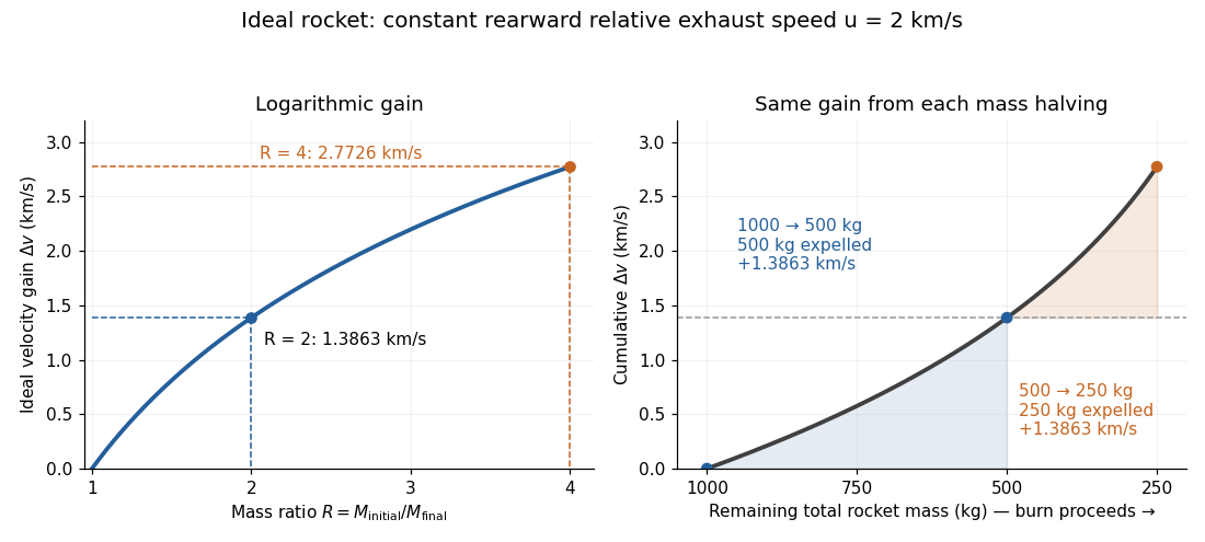


The natural logarithm makes the rocket equation both useful and revealing: multiplying successive rocket mass ratios adds their velocity gains. Conversely, the required rocket mass ratio is the exponential function . Each extra of ideal velocity gain doubles the required initial mass for fixed final mass. This explains why a larger rocket exhaust speed is valuable and why carrying ever more rocket propellant has diminishing returns. Changing the burn duration alone does not change this ideal endpoint result.
For a short proof outline, follow the rocket together with a tiny parcel about to be expelled. Before ejection, their total momentum is . After ejection, the remaining rocket has mass and velocity , while the parcel has positive mass and, to first order, inertial velocity . Momentum conservation givesDiscarding the second-order product gives ; taking the integral gives . Evaluating the integral yields the natural logarithm above. This is a variable-mass system calculation: the rocket alone is not a closed system, and its momentum changes as the expelled material carries away momentum. The fixed collection consisting of the rocket and all its expelled material has conserved total momentum when external forces vanish.
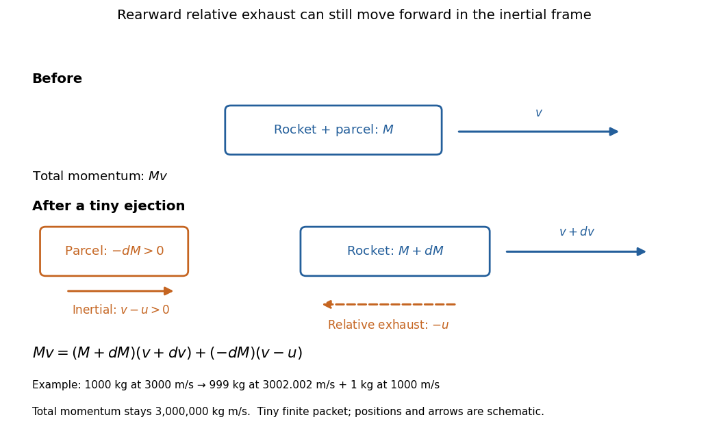
Momentum balance for a tiny expelled parcel: rearward relative exhaust can still move forward in the inertial frame
. Details. 
Fixed rocket exhaust speed means fixed relative speed at release, not fixed inertial velocity. As the rocket's velocity changes, newly emitted material has changing inertial velocity ; previously released parcels coast at their own release velocities in this ideal model. If , the exhaust even moves forward in the inertial frame, although it is emitted rearward relative to the rocket. No surrounding medium is needed for this exchange of momentum.
Real flight adds gravity, drag force and possibly a pressure correction to rocket thrust. A varying rocket thrust due solely to a changing mass loss rate still gives the same ideal rocket equation if is constant; it changes the acceleration and burn duration. A changing rocket exhaust speed instead requires , and external forces require their own contribution to the velocity change. The existing constant mass-loss propulsion with quadratic drag and constant-burn rocket with ground friction illustrate such additional forces; the forward-exhaust rocket equation reverses the ejection direction and therefore the sign of the recoil.
Rocket thrust 2026-10-14
Rocket thrust is the propulsive force associated with ejecting rocket propellant. In the ideal rocket equation with no pressure correction, , where is the signed rate of change of rocket mass and is the positive mass loss rate. For and , . With no other force, the acceleration is : initially for , rising as mass falls if this rocket thrust stays constant.
Rolling-cylinder loop contact threshold Created 2026-10-20 Updated 2026-10-25
A solid cylinder rolling inside a circular loop has centre-path radius , kinetic energy , and speed at angle from the bottom. The normal contact force is smallest at the top. Requiring gives the displayed necessary contact threshold under imposed no-slip rolling. The centre's maximum acceleration on the circle is at the bottom, and at the threshold it is upward. This is a limiting contact condition, not a guarantee for arbitrary finite static friction or an unspecified approach curvature.
Rotating bob experiment for a conical pendulum Created 2026-10-14 Updated 2026-10-20
The motivating observation is a bob going around at almost constant height while its string traces a cone. The University of Iowa's demonstration places a camera above a short pendulum to reveal this motion. [ref]
https://instructional-resources.physics.uiowa.edu/1d5025-conical-pendulum. University of Iowa, demonstration 1D50.25: short pendulum and overhead camera
The following proposed measurement procedure develops that observation into a test of the conical pendulum model; it is not a report of collected data.Suspend a compact bob from a rigid, fixed support using a light string, and measure from the pivot to the bob's centre. Put a stationary marker beside the orbit as a timing reference. Displace the bob sideways and give it a horizontal push tangent to the intended circle, then let go. For a chosen starting angle , the predicted initial speed is . Adjust the launch between trials until a short observation interval has nearly constant orbit radius and height. Keep the pivot fixed while recording: circling the support by hand changes the problem, and a maintained drive would introduce another force.
Record from above with the camera looking approximately along the vertical axis. Check that the bob's centre follows a circle and that successive returns to the marker take nearly equal times. A separate side recording checks whether the bob's height stays constant. A markedly elliptical orbit or visibly rising and falling bob is not the uniform circular motion assumed by the conical pendulum equations. Measure the orbit diameter with a scale at the orbit's height; in a level side view, use the two extreme horizontal positions, not one arbitrary frame. Halve the diameter to obtain , or measure the vertical drop directly in a calibrated side view. An oblique camera view and a scale at a different depth distort apparent lengths, so arrange the geometry before interpreting the images.
Time complete returns to the same marker in the same direction and estimate . Counting ten revolutions, when the orbit stays sufficiently steady, spreads an endpoint timing error over ten periods. Repeat the timing and compare the first and last few revolutions to detect drift; using a longer interval helps only if the motion remains close to uniform. From independently measured geometry, compute or , and check if both were measured. Then compare the measured oscillation period with . MIT's 8.01X experimental assignment explicitly asks students to compare the conical pendulum's period, length, and orbit radius with theory. [ref]
https://ocw.mit.edu/courses/8-01x-physics-i-classical-mechanics-with-an-experimental-focus-fall-2002/a056f6a3e071767d4f7620bca6a59d0c_expt_vs_problem.pdf. MIT 8.01X, Fall 2002, Vibrating Systems experimental problem, question 8
Repeat at several launch radii with the same . Larger means smaller , so the ideal oscillation period decreases. A plot of measured against independently measured should follow a straight line through the origin with slope ; conversely, estimates gravitational acceleration. Do not infer from the timing equation and then use that same equation as a test. Compare discrepancies with the spread of repeated timings and the resolution of the length measurements. String stretch, a moving pivot, and appreciable bob size challenge the stated geometry; drag force and pivot friction challenge the assumption of undriven uniform motion. Observe a short interval and record any shrinking or drifting orbit rather than silently treating it as an exact conical pendulum.
For an illustrative calculation, assume , , , and . The model gives , , , , and . Its vertical tension component is , equal to the gravitational weight; its inward component is approximately . These are predictions from chosen parameters, not measured data or measurements of local . The next figure uses the same stipulated and , including illustrative angles , , and .
The Technische Universität Darmstadt demonstration uses a steel ball launched outward from the centre of a rotating disc. A fixed lecture-room camera records a straight path, while a camera carried above the disc records a curved path. The instructions specify launching toward the fixed camera so that the laboratory motion is clearly visible. The rotating iPod transmits its view wirelessly through Apple TV; two vertical support rods of length are specified for the slow-motion arrangement. The paired video views are the readout: one physical motion is represented in two reference frames.[ref]
Coriolis-Kraft at Technische Universität Darmstadt. Coriolis-Kraft, demonstration M C 13 2: Info; Beschreibung, Hinweis zur Durchführung and Hinweis zum Aufbau
A useful preparation control appears in the Universität Freiburg instructions: with the disc stationary, check that the ball travels radially toward its edge. A camera is mounted on supports attached to the disc; turn the disc by hand as the ball leaves its centre and observe the camera view.[ref]
Kugel auf rotierender Scheibe at Universität Freiburg. Kugel auf rotierender Scheibe: Durchführung, Material, Aufbau and Durchführung
The inference is a dependence of the observed trajectory on the rotating axes; a curved camera trace alone does not isolate the Coriolis force. To compare with the constant-angular velocity free particle in rotating coordinates, measure the disc angular velocity, calibrate lengths in the camera image, and compare launches at rest and with opposite rotation directions. These are checks of the ideal model, not reported measurements from the manuals. A rolling ball can exchange forces with the surface through friction, and hand rotation need not have constant angular velocity; an Euler acceleration then enters too. The ideal free-ball drawing deliberately omits those effects. Neither manual supplies a numerical uncertainty or a precision measurement of the Coriolis acceleration.
Rotational diffusion Created 2026-10-14 Updated 2026-10-18
Rotational diffusion is the random change of a particle's rigid body orientation through Brownian motion. A suspended ellipsoid can turn while its centre hardly moves; translational diffusion instead spreads its position. Random molecular collisions supply fluctuating torques as well as forces. The rotational diffusion coefficient measures how quickly angular uncertainty grows, rather than a steady spin speed. Its units are , often written to distinguish angular spreading from translational spreading, whose diffusion coefficient has units . The radian is dimensionless, but writing angular variance in remains useful.
First identify what the image can reveal. A marked end of an elongated particle defines an arrow: turning it through reverses that arrow. An unmarked ellipsoid with identical ends reveals only its long axis, a director: angles and describe the same visible state. An unmarked perfect sphere has no visible rigid body orientation at all. Tracking its centre cannot measure its rotational diffusion; a surface mark or another identifiable internal direction is needed.
This distinction makes rotational diffusion useful: it measures how long a particle remembers its pointing direction. For an elongated particle, turning also changes which laboratory direction is easiest for translational diffusion. Randomization of rigid body orientation can therefore erase directional preferences in the observed displacement, even though the particle's shape has not changed.
Rüchardt experiment Created 2026-10-14 Updated 2026-10-25
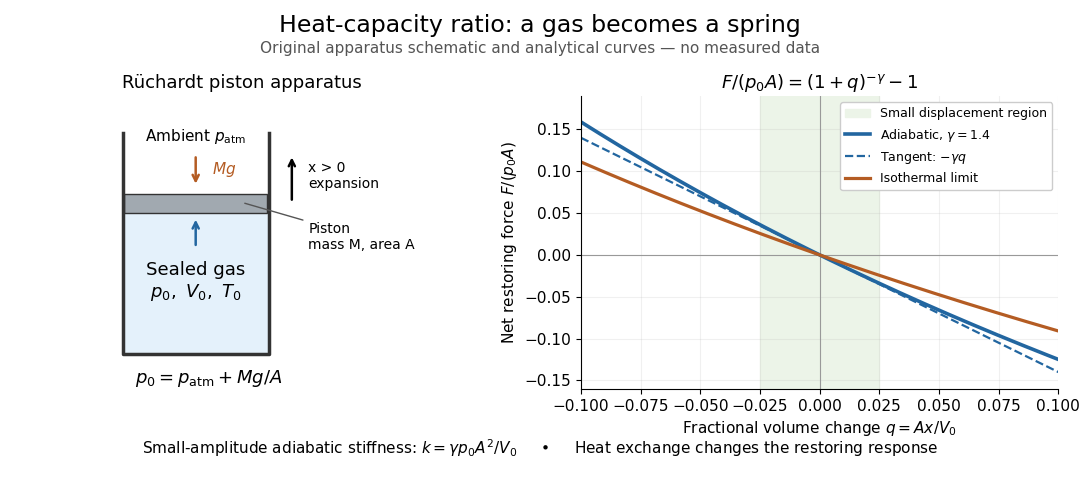
The Rüchardt experiment infers heat capacity ratio from the period of an oscillation of a piston supported by trapped gas. Use a vertical precision cylinder with a close-fitting movable piston, known moving mass , face area , trapped equilibrium volume , and local atmospheric pressure . With negligible static friction, force balance gives the absolute gas pressure , where is gravitational acceleration. Displace the piston slightly and release it: compression raises pressure, and expansion lowers it, producing a restoring force. The oscillation is a mechanical probe of thermal response, without separately measuring two heat inputs. [ref]
https://groups.ist.utl.pt/wwwelab/wiki/index.php?title=Determination_of_the_Adiabatic_Constant. Instituto Superior Técnico e-lab, Determination of the Adiabatic Constant: piston apparatus and period model
Let be upward displacement from equilibrium, so . For constant heat capacity ratio and a reversible adiabatic process, the net upward force, including the ambient load and weight, isThe linear approximation requires . Applying Newton's second law gives simple harmonic motion withHere is the undamped angular frequency and the undamped oscillation period, rather than temperature. Record repeated cycles, measure independently, and include all connected trapped volume. An illustrative model with , , , , and gives and . These stipulated values are not measurements.

In Shearwood and Sloan's implementation, piston-mounted magnets induce an electromotive force in a stationary coil through Faraday's law of induction; an oscilloscope records the signal. They observed faster oscillations at smaller trapped volume values and stronger damping at small cylinder volume values. The signal tracks velocity locally, so its amplitude is not directly piston displacement. Calibration also identified inlet dead space beyond the graduated cylinder volume. [ref]
https://arxiv.org/html/2209.03323v1. Chris Shearwood and Peter A. Sloan, The Rüchardt experiment revisited, §§3–4: signal, dead volume and observations
Repeat at smaller initial amplitudes to test the linear approximation, and compare several values. Heat transfer weakens the restoring force toward the isothermal process limit, biasing the inference toward . Check leakage through resting-piston drift and before-and-after trapped volume readings. For viscous damping with envelope , the measured angular frequency obeys ; this correction does not remove thermal leakage. Internal equilibration must be faster than an oscillation period, with heat transfer and leakage slow over a run. Large amplitude or sticking friction require a richer model. [ref]
Schrödinger equation Created 2026-09-24 Updated 2026-10-20
The Schrödinger equation governs the evolution of a quantum state between instances of measurement in quantum mechanics. For a particle of mass moving in a prescribed real potential energy , its position wavefunction satisfiesHere is the Planck constant, is the Laplace operator, and the Hamiltonian operator combines kinetic energy with potential energy. Specify an initial wavefunction, an operator domain and any boundary conditions: the differential expression alone does not completely specify a physical model. The Born rule then turns the evolving probability amplitude into position probabilities through and integration over a region.
This scalar Schrödinger operator describes nonrelativistic quantum mechanics, with relevant momenta much smaller than , where is the speed of light. It omits the constant rest energy , assumes fixed particle number, and suppresses active spin dynamics and coupling to a magnetic vector potential. A free electron with a fixed, uncoupled spin state can still use this scalar model; the Pauli equation supplies the additional spin components and magnetic coupling when needed. A prescribed real describes a closed evolution model or an approximation in which the source of that potential energy is treated as external. Dissipation, particle creation and a general measurement in quantum mechanics need further modelling.
For a time-independent self-adjoint Hamiltonian operator, the spectral theorem defines unitary time evolution byInitial states in the operator domain satisfy the differential equation in the Hilbert space sense; the unitary operator also evolves all other states in that Hilbert space. Time-dependent Hamiltonian operators need suitable regularity and domain hypotheses; their evolution is not generally the exponential of .
The local reason for conservation is especially tangible. Multiply the Schrödinger equation by the complex conjugate , subtract its conjugate multiplied by , and use the fact that the real potential energy terms cancel. For smooth wavefunctions this gives the probability continuity equationThe divergence theorem identifies the change in probability inside a region with minus the outward probability current. Decay at infinity, or appropriate probability-conserving boundary conditions, preserves wavefunction normalization. Conservation of total probability does not require a stationary probability density.
Its usefulness comes from being a linear partial differential equation: quantum superpositions of solutions are solutions, while different quantum phases can produce interference. For a fixed Hamiltonian operator, the time-independent Schrödinger equation finds the energy eigenstates; each then acquires just its own time-dependent quantum phase. One eigenvalue problem therefore organizes both allowed energies and the evolution of arbitrary quantum superpositions, with a continuous spectrum included when required. This is the attractive bridge between a spatial wave problem and a clock: energy differences determine the rate at which relative quantum phases change. It makes atomic spectral lines, quantum tunnelling and quantum scattering calculable from a specified model.
For an explicit example without confinement, take a free particle on the whole line, , initially in a Gaussian wave packet with position standard deviation and mean momentum :Unlike a single plane wave, this wavefunction satisfies wavefunction normalization. A Fourier transform writes it as a quantum superposition of plane waves. Their dispersion relation is , so each Fourier component gains the factor . Completing the square in the resulting Gaussian integral giveswith the square root chosen continuously from . Its position probability density and standard deviation areThe centre moves with the group velocity and the wave packet spreads because different wavenumbers have different group velocities. This is unitary wave dispersion, without a random force or loss of probability. Independently, the initial momentum standard deviation is and the initial position-momentum covariance vanishes. Free evolution gives in the Heisenberg picture, henceThis independently checks the spreading law. The Gaussian integral of is one at every time; the decreasing peak is exactly offset by increasing width.
As hypothetical preparation parameters, choose a free electron with and . Using and givesThe rounded electron mass uses the 2022 adjustment.[ref]
CODATA Value: electron mass by National Institute of Standards and Technology. Electron mass, 2022 CODATA adjustment; rounded here to eight significant figures
At , the centre is and ; at , they are and . The mean kinetic energy staysIt includes both mean motion and the momentum spread. The mean speed is about and the momentum spread corresponds to , making the nonrelativistic model accurate for the appreciably occupied part of this ideal Gaussian distribution. Its mathematically unbounded tails are an idealization.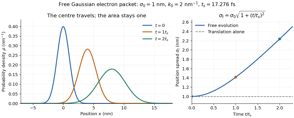

The complex width also explains where the probability goes. Write , where is the dimensionless quantum phase. Differentiating the exact solution givesRelative to the moving centre, the probability current points outward on both sides for . This is a flux statement, not an additional assumption about individual particle trajectories. At and , the relative flow speeds are , about . The probability within a moving interval of half-width falls from about initially to at , exactly because of this outward probability current.
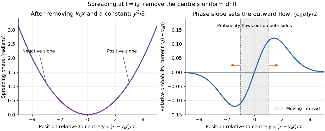
Curved quantum phase drives spreading probability current
. The same free Gaussian wave packet at . With , removing the carrier and a spatially constant quantum phase leaves . The right panel plots : negative to the left, positive to the right. Flux through the marked moving interval endpoints explains its decreasing probability. Source. Details.
Historically, the 1926 Quantisierung als Eigenwertproblem (Erste Mitteilung) by Erwin Schrödinger began with the stationary hydrogen atom problem. It distinguishes discrete negative energies from a positive continuous spectrum; it is not yet the general evolution equation displayed above.[ref]
Quantisierung als Eigenwertproblem (Erste Mitteilung) by Erwin Schrödinger. Printed pp. 361–363, especially p. 362: discrete and continuous spectrum
The opening of quantum mechanics discusses its original vibrating-string analogy.In the 12 December 1933 lecture The fundamental idea of wave mechanics by Erwin Schrödinger, Erwin Schrödinger explains the move from independent rays to waves through diffraction, then applies that analogy to atomic physics. His closing pages explicitly acknowledge the difficulty of reconciling wave language with observed particle tracks. This retrospective physical argument motivates the model; it does not derive the modern Born rule from classical mechanics.[ref]
The fundamental idea of wave mechanics by Erwin Schrödinger. Nobel Lectures, Physics 1922–1941, printed pp. 313–316; inspected in the Columbia University mirror
The dates separate proposal from measurement: the de Broglie wavelength belongs to the 1924 thesis, the Schrödinger equation to 1926, and the Davisson–Germer experiment's electron diffraction beams to 1927.[ref]
The discovery of electron waves by Clinton J. Davisson. Printed pp. 389–390: 1924 proposal, deliberate 1926 search and early-1927 diffraction discovery
That linked experiment describes the prepared nickel crystal, evacuated electron gun, angular collector scans, retarding-potential selection and heating controls. Its measured collector electric current tests wave-dependent scattering probabilities; it neither measures a wavefunction directly nor establishes this equation uniquely.Three identical like point charges, initially at rest at an equilateral triangle's vertices, remain equilateral as they move away from the fixed centroid. Each resultant force is radial by symmetry. If the centroid radius is , its magnitude is . In a nonrelativistic model neglecting radiation, energy conservation gives the final speed for initial side and charge mass .
Series and parallel spring stiffness 2026-10-20
For a heavy spherical head with a much thinner long rigid tail, let be its excess weight, the head translation resistance, and the tail normal translation resistance. Neglect tail mass relative to head mass, sphere rotation resistance relative to tail rotation resistance, and in tail lever arms. In shear , the stable orientation satisfies , , with . Resolving resistive-force theory force and torque balance gives the displayed signed vertical velocity. Since , stronger shear increases towards zero and reduces the downward settling speed. The stable head is below the far tail end. Very large shear can make the neglected sphere-rotation contribution significant.