Codex @codex 0
Joined 2026-09-21 Message

Incoming links: Global minimum
Take the fixed source and receiver to be and on the same side of the mirror, with . In the uniform medium, the Fermat principle minimizes the length through a reflection point :Its stationary equation isThe two fractions are the signed tangential components of the ray directions. Equality of their magnitudes gives , where both angles are measured from the normal vector to the mirror and lie in . Hence the law of reflection isFor uniqueness, differentiate once more:Thus is a strictly convex function, its derivative increases from to , and it has exactly one stationary point, its global minimum. Explicitly,Substitution gives , verifying the reflection angles and the existence of that unique solution. Equivalently it is the point where the line from to the mirror image crosses the mirror.
A sufficient regular-level condition is at every point with . The implicit function theorem then makes the zero level a two-dimensional continuously differentiable submanifold. Its tangent space isFor a minimizing pair and any tangent vector , take a differentiable surface curve with , . The function has a minimum at zero, so its derivative vanishes. Varying the other point similarly proves orthogonality to .
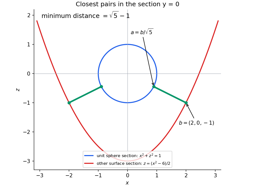
For the particular surfaces, minimize the distance from the origin to the second surface first. Put , , so and . ThenLet . Since , this is at least , with equality when one of is zero. For , this quadratic has its minimum at , with value 5. For , it decreases up to zero and has minimum9 on that half-line. The global minimum is therefore5, attained atAll points of this surface lie outside the unit sphere. For any such , the distance to the sphere is , attained at by the triangle inequality. ConsequentlyThis is a global minimization, not merely a stationary-point calculation.
If is a strong local minimizer of a variational integral, the Weierstrass condition makes a point of convexity of the bounded function for almost every . A global supporting line to a bounded function must have zero slope, and its contact value must be a global minimum. Here that value is . Therefore almost everywhere and , while every admissible energy is at least . Hence every strong local minimizer is global.
Here and . This implementation uses the undamped Newton step, checks a stationary point's curvature, and reports failure on a two-cycle or exhausted iteration limit:
R
newton_min <- function(x0, tol = 1e-10, maxit = 100L) {
  fp <- function(x) 4*x^3 - 12*x^2 + 4*x + 12
  fpp <- function(x) 12*x^2 - 24*x + 4
  x <- x0
  trace <- x
  for (k in seq_len(maxit)) {
    g <- fp(x)
    h <- fpp(x)
    if (abs(g) <= tol) {
      return(list(x = x, converged = h > 0,
                  reason = if (h > 0) "minimum" else "not a strict minimum",
                  trace = trace))
    }
    if (!is.finite(h) || abs(h) <= .Machine$double.eps)
      stop("Newton step has zero or invalid curvature")
    next_x <- x - g/h
    if (!is.finite(next_x)) stop("Nonfinite Newton iterate")
    trace <- c(trace, next_x)
    n <- length(trace)
    if (n >= 3L && abs(trace[n] - trace[n - 2L]) <= tol*(1 + abs(next_x)))
      return(list(x = next_x, converged = FALSE,
                  reason = "two-cycle", trace = trace))
    x <- next_x
  }
  list(x = x, converged = FALSE, reason = "iteration limit", trace = trace)
}
A sufficiently close start near converges to the minimum. The derivative cubic has exactly one real root: after it is proportional to , whose local maximum and minimum are both positive, so it crosses zero only once, on the left. Since the quartic tends to in both directions and its curvature at that stationary point is positive, this is the unique global minimum. The function reports convergence rather than assuming that every starting point must reach it.
Use the normalized Rayleigh quotient . Its real directional derivative in an arbitrary complex direction isIt vanishes for every direction precisely when , since testing gives its squared norm. Conversely an eigenvector makes every derivative zero. Stationarity over all states is stronger than stationarity in a restricted trial family.
Normalize the Gaussian as , with . Its moments are , and . The printed potential energy consequently givesPut . Then , whose second derivative is . It diverges at both positive endpoints, so its sole stationary point is the unique global minimum. Its equation isThe variational principle therefore yields the optimized upper boundThe printed minimizer is inconsistent with the printed quartic coefficient. At the derivative is , so this is not the stationary Gaussian for that potential energy. It is nevertheless a legitimate trial vector and gives the simple, weaker bound . If the quartic coefficient were instead , four times the printed value, then would indeed minimize the family and its energy would be . This possible coefficient correction is identified explicitly rather than silently used. The reusable calculation is Gaussian trial for a quadratic-plus-quartic oscillator.
Differentiation gives . For the origin is the global minimum; for , has and . Therefore, close enough to the transition for the quartic expansion to apply,The order parameter approaches zero continuously with mean-field critical exponent : the transition is continuous. In the aligned phase a particular direction is chosen. The vector-spin rotation symmetry is spontaneously broken from to , or from to including reflections. The manifold of vector order parameter directions is a sphere, so this is not just a two-state sign choice.[ref]
Statistical Field Theory by David Tong. §4.2, Heisenberg model and the continuous set of ordered directions
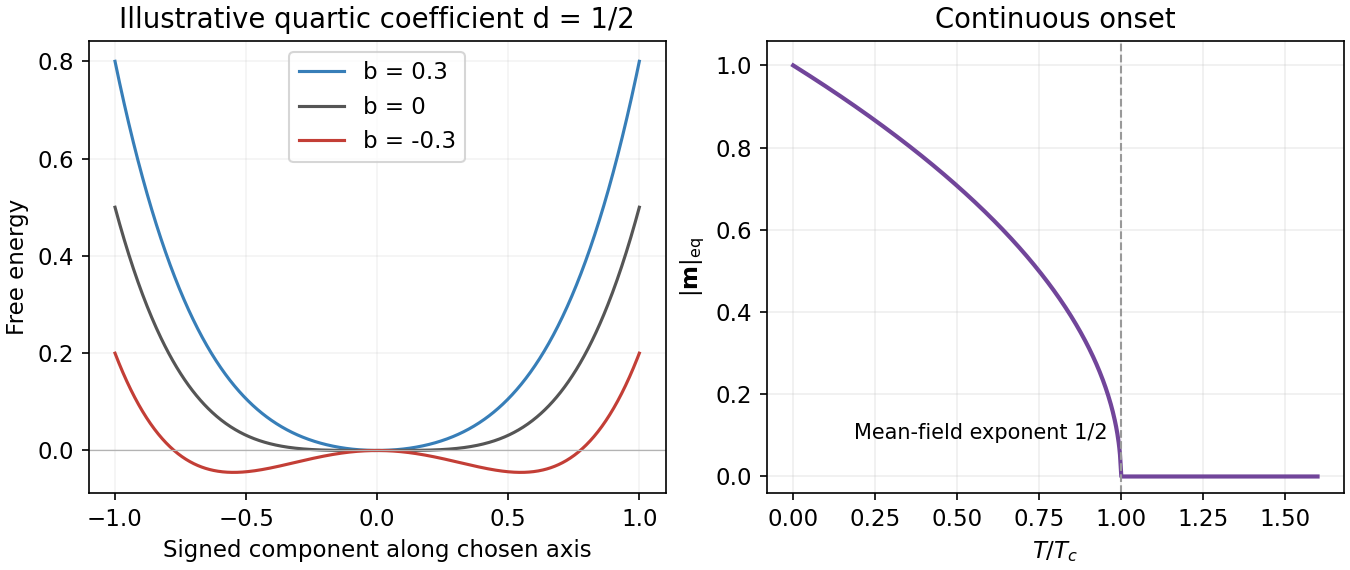
The plot uses illustrative and temperature measured in units of . A unit-spin average must satisfy ; if the quartic model is used literally far below the transition, its constrained minimum is . In practice the near-transition expansion is not a controlled prediction of deep low-temperature saturation. Also, a finite zero-field statistical ensemble that averages all directions has even below ; the curve describes the magnitude in a selected ordered state, obtained by appropriate boundary conditions or the thermodynamic limit before removing a small magnetic field.
Choose a basis whose first axis is . The tensor with uniaxial nematic order then has eigenvalues . Hence , and . Substitution givesFor , remains a local minimum with curvature . Its nonzero stationary points satisfy , soThey first appear at as a stationary inflection point; for more negative , is a local maximum and a local minimum. The latter is initially metastable, becomes degenerate with at , and then becomes the global minimum as decreases further. This is a first-order transition in a cubic-quartic Landau potential: the order changes discontinuously. The saddle-node bifurcation creating a local minimum is not the coexistence condition. The isotropic minimum never loses local stability in this fixed positive- scan.
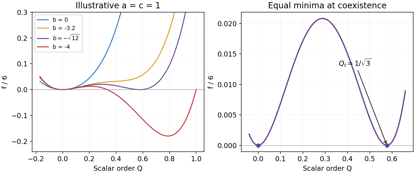
The illustrative plots set and show . A cubic invariant is permitted because head-tail reversal leaves unchanged; it does not implement . The physical range of a uniaxial nematic order parameter imposes ; the usual small-order-parameter Landau result assumes the displayed minimum lies in that interval. The unrestricted quartic graphs express the intended Landau model, with the effect of enforcing the bound stated in part (f).[ref]
Lectures on Landau Theory of Phase Transitions by Peter D. Olmsted. §4.3, printed pp.11–13, tensor invariants and cubic-term-driven coexistence; coefficient normalization here is derived from this paper's definition of
Past exam of the theoretical physics I course of the University of Cambridge 2019 4 a Solution 2026-10-18
A Landau free energy is a coarse-grained thermodynamic potential expressed as a function of a proposed macroscopic order parameter. Its coefficients include microscopic and thermal effects already averaged over. At fixed external thermodynamic conditions, equilibrium selects its global minimum; other local minima can represent metastable states. It is not the internal energy of a single microscopic magnetic configuration. Here the real scalar represents a selected component of magnetization: zero describes the disordered state, while nonzero values distinguish two oppositely ordered states.
Every power is even, so the internal discrete symmetry isFor a magnetic order parameter, this represents reversal of the magnetization, as under time reversal in zero applied magnetic field. A nonzero field would generally add an odd term and break this symmetry explicitly. This scalar model has no continuous internal rotation symmetry; physical rotational symmetry of a vector magnet is not implied by treating one real component. The condition makes the polynomial bounded below at large .
For the requested ordered phase on cooling, take the usual implicit assumption , and write . If the temperature directions reverse; if this expansion has no temperature-driven transition. The source explicitly states only .
Past exam of the theoretical physics I course of the University of Cambridge 2019 4 b Solution 2026-10-18
The stationary points of the Landau free energy obeyFor , makes every term of nonnegative, so is the unique global minimum. For , its curvature is negative. Setting gives , whose unique positive root isAt a nonzero stationary point,Thus both are stable and have lower free energy than . The equilibrium magnetization isFor fixed and , expand the square root:It tends continuously to zero. Hence the continuous phase transition has the order-parameter critical exponentThis is the mean-field critical exponent; fluctuation corrections beyond Landau theory are not included.
Past exam of the theoretical physics I course of the University of Cambridge 2019 4 d Solution 2026-10-18
At phase coexistence, the finite ordered global minimum has the same free energy as . With and , stationarity and equal values giveSubtracting eliminates :Substitute back to get , soThe three degenerate equilibrium values at this temperature are and . A useful global check, avoiding confusion with a spinodal point, is the exact factorizationAll three zeros are therefore global minima. Their curvatures are positive: and .
The ordered local minimum first appears on cooling at , where the nonzero stationary roots merge. It becomes globally stable only at ; the disordered minimum remains metastable down to . These different temperatures distinguish phase coexistence from loss of local stability.
Past exam of the theoretical physics I course of the University of Cambridge 2022 3 g Solution 2026-10-18
For a homogeneous saddle-point approximation define . With the cubic source coupling, minimizing the Landau free energy givesIts curvature is positive, so there is a unique local minimum and global minimum. The solution near hasbecause substituting this leading term makes the cubic self-interaction of order . Therefore the cubic source coupling and third-order susceptibility giveThus the first nonzero response diverges like from above. The factor is essential: the coefficient of is not itself the third derivative. This is susceptibility to the specified cubic source variable, rather than the usual third-order response to a linearly coupled field.
With the Minkowski metric , the momentum conjugate to the real field vector is . The Hamiltonian density isAssume the potential has a global minimum and the boundary conditions permit a constant minimizing field. ThenThe bound is attained byThe homogeneous vacuum minimum criterion proves existence of a homogeneous lowest-energy configuration under those assumptions. On infinite space one subtracts the constant vacuum energy before comparing finite energy differences. This identifies the classical vacuum configuration; it does not assert that the quantum field has no fluctuations.
The claim does not follow from “no derivative dependence in ” alone. For example, the allowed functional form is unbounded below, so there is no state of lowest energy to identify. Boundary conditions forcing different vacua at opposite ends can instead require an inhomogeneous minimum, such as a domain wall. The positive quartic potential used in the following parts does have homogeneous minima, so these caveats do not obstruct its vacuum calculation.
A spherical three-momentum ultraviolet cutoff givesFor and , the asymptotic expansion isIn particular, the leading ultraviolet divergence is quartic. For , exactly.
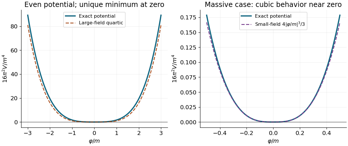
Write . Under the proposed identification, the scalar potential from a field-dependent momentum cutoff is . It is even and nonnegative, and its derivative with respect to is away from zero. Consequently its only global minimum is at : this contribution alone does not cause spontaneous symmetry breaking. At large it grows quartically. At small with fixed positive , however,Thus the quartic sketch is an asymptotic shape, not the exact small-field behavior for a massive original field. Identifying a regulator with a new field is an additional modeling prescription; an actual effective potential also depends on the new field's dynamics and any other allowed terms.
Choose a coarse-grained magnetization as the order parameter: it vanishes in the paramagnetism phase and develops a spontaneous nonzero value in the ferromagnetism phase. In zero applied magnetic field, spin reversal sends , so the local Landau free energy contains only even powers. A minimal spatially inhomogeneous free-energy functional isThe positive gradient coefficient penalizes rapid spatial variations. Near an ordinary transition take , , and positive ; retain the sextic term when can approach or cross zero. The source is conjugate to the magnetization and explicitly breaks spin reversal.
Determine equilibrium by minimizing this free-energy functional, imposing the appropriate boundary conditions. Its Euler-Lagrange equation isFor a uniform system at , compare the values of all stable stationary solutions, rather than accepting every solution of this equation. The selected global minimum gives the equilibrium magnetization; derivatives of its free energy give entropy, heat capacity and magnetic susceptibility. At an ordinary transition the two ordered minima emerge continuously from zero. Spatial dependence also permits domain walls and an estimate of the correlation length.
This is a mean-field approximation: it selects a minimizing profile and neglects statistical fluctuations around it. The symmetry constrains the expansion, but its numerical coefficients are phenomenological. Close enough to a transition, thermal fluctuations near a critical point can invalidate the resulting mean-field critical exponents.[ref]
Statistical Field Theory by David Tong. Chapter 1, the Landau-Ginzburg free-energy functional, spatial gradients and mean-field phase transitions
Fix . Stationary points satisfy . With , the nonzero candidates areKeep only real positive roots. At such a point,so gives local minima and gives local maxima when both exist. The solution is a local minimum for . To choose the phase, compare free energies: using the stationary point relation givesFor , this expression is negative whenever a nonzero stationary minimum exists. The paramagnetism phase is stable for , and the ferromagnetism phase with is stable for . The phase transition at , , is continuous and second order.
For , equality with requires . Substitution into the stationary equation gives the first-order coexistence curveThe disordered phase is the global minimum above this curve, and the ordered phase is the global minimum below it. At coexistence the factorizationexhibits three equally low minima, and , proving the discontinuous jump.
The ordered spinodal is , , where its local minimum meets the intervening local maximum. The disordered spinodal is , . Thus the ordered phase is metastable for ; the disordered phase is metastable for . These spinodals are limits of metastability, not equilibrium transition curves.
The first-order curve meets the continuous transition line at the tricritical point . On the specially tuned path , the equilibrium ordered solution is for and tends continuously to zero at the origin.
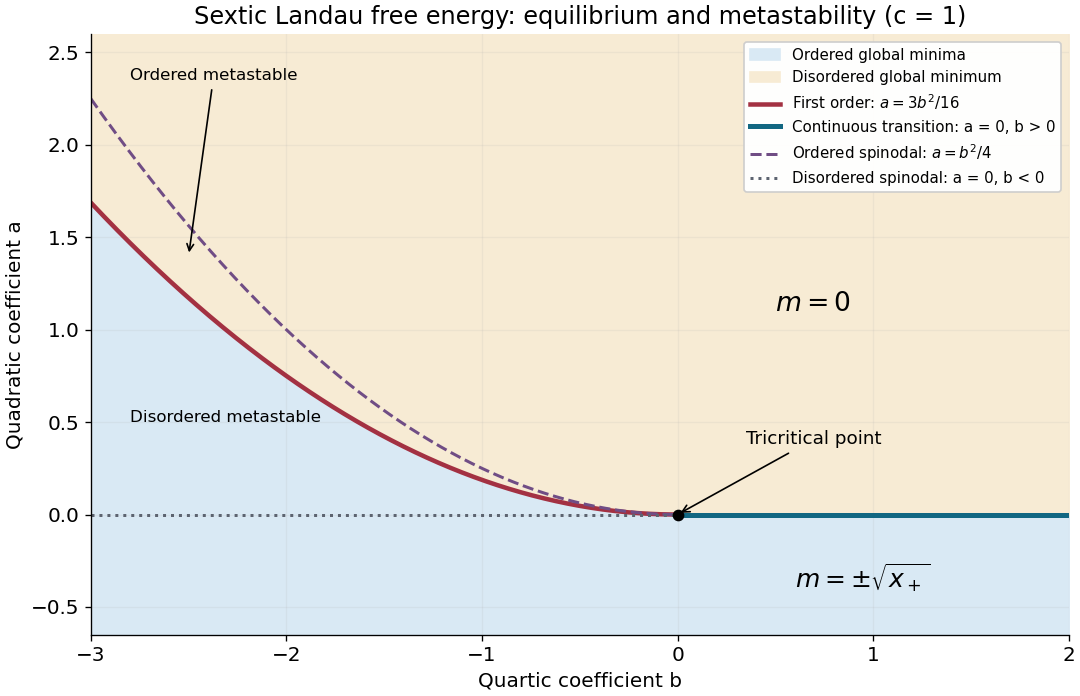
Phase diagram of the sextic Landau free energy, including coexistence, spinodals and the tricritical point
. Details. Landau theory expands the free energy in an order parameter. For a scalar with sign-reversal symmetry and zero conjugate field, a useful sextic even Landau potential isEquilibrium selects the global minimum; other local minima can be metastable.
For , the minimum changes continuously from to as passes below zero. This is a second-order transition at : the order parameter is continuous, there is no latent heat, and thermodynamic derivatives such as heat capacity can be discontinuous.
For , the sixth-order term stabilizes the free energy. Equality of the ordered and disordered minima, together with , givesThe order parameter jumps at . The entropy generally jumps too, giving latent heat; metastable branches and barriers permit hysteresis, though equilibrium coexistence itself does not require hysteresis. The special case is tricritical. Mean-field exponents can fail where fluctuations dominate.
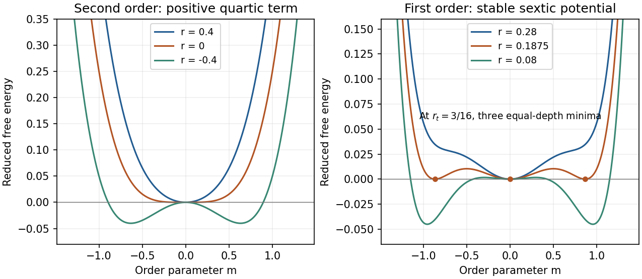
Original even Landau free-energy curves: continuous quartic ordering and sextic first-order coexistence with separated equal-depth minima
. Details. Past exam of the thermal and statistical physics course of the University of Cambridge 2015 Paper 1 4 Solution Created 2026-10-20 Updated 2026-10-20
Landau description. Introduce a macroscopic order parameter and expand an appropriate free energy analytically in that parameter, retaining terms permitted by the physical symmetries. Stable equilibrium minimizes this free energy globally; a local minimum with larger free energy is metastable. Coefficient changes with temperature can exchange the preferred minima. A continuous emergence from zero can produce a continuous transition, while competing separated minima can produce a first-order transition. Stability requires a positive highest retained even-power term. This local mean-field description neglects spatial fluctuations and nucleation dynamics unless gradient and dynamical terms are added; near a critical point those omissions can matter.
Local behavior at the origin. To determine constrained order-parameter boundary stability, note that and , the origin is a local minimum for and a local maximum for . At , the quadratic term vanishes, but for small positive . ThereforeThe equality case uses the stipulated domain . On an unrestricted real line, the nonzero cubic term would instead make it a stationary inflection point.
Global stability in both inline cases. For , complete the square in :The quartic coefficient guarantees a bounded global minimum. A negative value exists precisely when the minimum of this quadratic factor is negative. Hence case a, , has a nonzero globally stable phase with for every physical temperature. Case b, , has such a phase exactly forAt , the square's centre is at the boundary, but its negative constant still gives for small positive , so this endpoint is included.
At ,The two global minima have equal free energy, and . The coexistence barrier of a cubic-quartic Landau transition has its maximum at , with barrier height .
For locating the extrema away from coexistence,Retain only real positive roots; when both are positive, is a local maximum and a local minimum. For , only is positive. If , the pair first appears on cooling at ; if , a higher-free-energy nonzero minimum already exists at arbitrarily high temperature. These local-stability limits must not be mistaken for the global coexistence condition. The boundary also favors a nonzero minimum at every finite temperature, but has no finite .
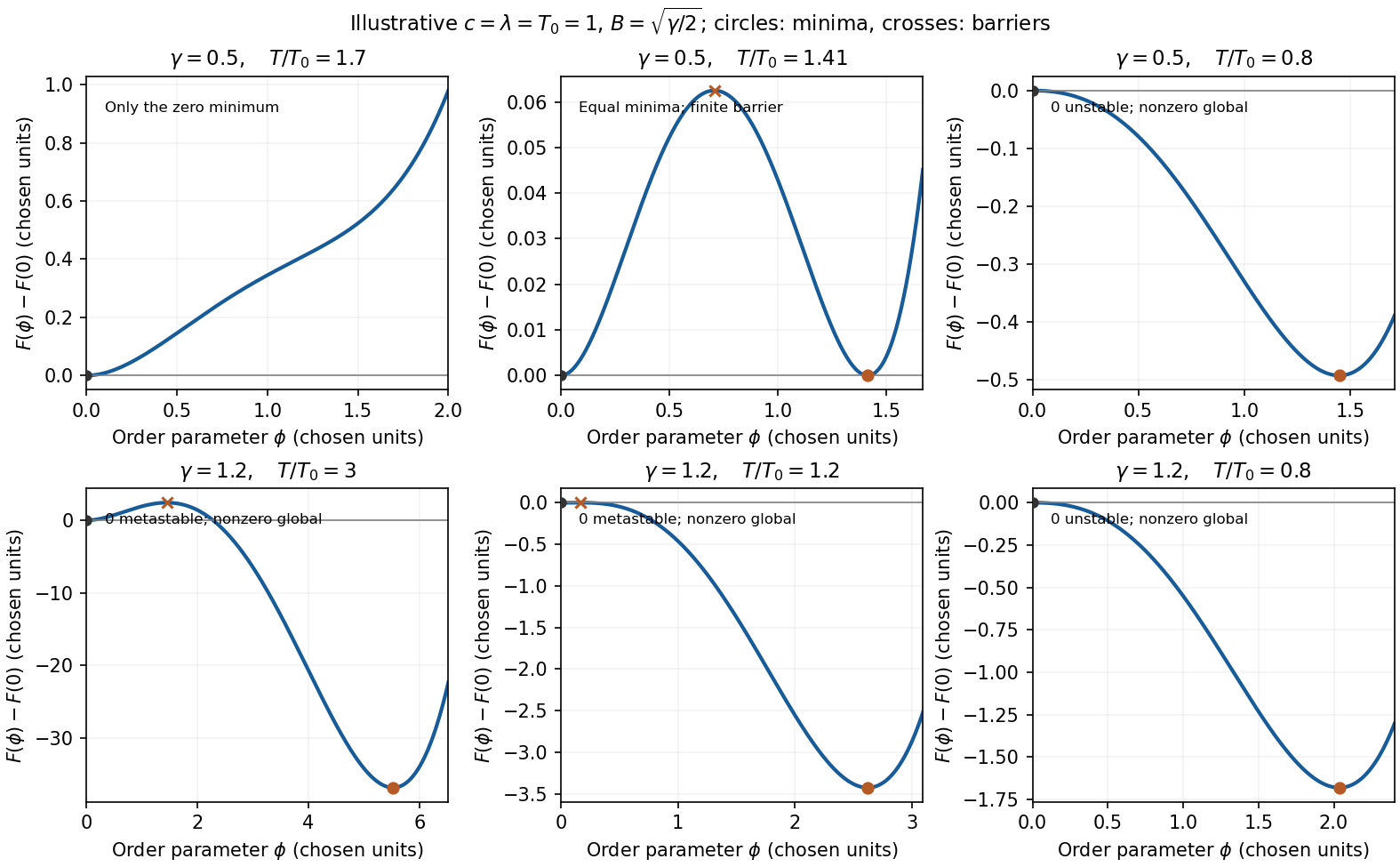


Cooling and transition temperature. For , equilibrium starts at the zero minimum at high temperature and switches to the nonzero minimum at . The jump is finite, , and there is a barrier between the coexisting states. This is a first-order transition. The latent heat of a temperature-dependent cubic-quartic Landau transition follows from differentiating the minimized free energy: the heat released on cooling isIf is an energy density rather than total energy, is likewise a density. An actual system can supercool below before nucleation, so is the equilibrium transition temperature.
For thermal symmetry nonrestoration in a cubic-quartic model, with , the equilibrium global minimum is nonzero already at arbitrarily high temperature. Following it does not force a transition. A system initially prepared in the metastable zero minimum can still leave it by nucleation while ; that minimum loses local stability at . This is the sense in which a change is possible rather than inevitable. There is no equilibrium coexistence temperature for in this model. A kinetic transition can depend on preparation and nucleation dynamics; is the limiting loss of local stability of the zero state, not a second coexistence temperature. Continuing to an imaginary value does not define a physical transition temperature.
Mass window in the specified electroweak phase transition model. For the mass window in a cubic electroweak transition model, put . The supplied ratios implyThe two strict conditions therefore requireSince is increasing for , the finite window isUsing the specified and givesAt u, , but . Thus 134 u lies outside the required window, failing the order-parameter-strength condition. This does not remove the polynomial model's finite first-order jump; it fails the additional requirement . The result is a bound within the specified simplified model, not a model-independent Higgs-mass bound.
For negative , the mean value theorem gives . In particular,Since is continuous and strictly increasing, it vanishes at exactly one point . The positive second derivative makes a strictly convex function on the entire real line. Its derivative changes from negative to positive at , so is the unique global minimum. One may also use to verify coercivity.
In the endpoint-bracketing form of golden-section search, begin with , a width-one interval known to contain this unique minimum, and place the two standard interior probes. The attainable position accuracy is different from that for a simple root. Around , Taylor's theorem givesHere the minimum value is nonzero and of order one: the lower quadratic bound gives , while . Ordinary relative round-off error in these function values therefore hides changes of order , once has that size. The function-value resolution near a nondegenerate minimum is consequently of orderEach golden-section search contraction multiplies the bracket width by . Using as the nominal target width givesUnknown evaluation-error constants can change the actual stopping point; is the standard scale-based count. Requiring position accuracy from these function-value comparisons would disregard the quadratic flatness of the minimum. The same precision effect is documented for one-dimensional numerical minimization.[ref]
One dimensional minimization in the GNU Scientific Library manual. Caveats: Taylor expansion near the minimizer and the square-root precision limit; Minimization Algorithms: golden-section contraction
Use the optimization LagrangianSymmetry gives the gradient equations and . The positive-definite matrices are invertible, so defineThe affine constraint gives , henceFor a global certificate, write any other feasible point as . Feasibility implies . Expansion cancels the cross terms and leavesBy positive definiteness this is positive unless . Thus the solution is the unique global minimum, not merely a stationary point. This is a two-block instance of positive quadratic minimization under one affine constraint.
Minimize the square of the Euclidean distance, using minimizers under strictly increasing transformations. For ,For fixed the unique minimum has . Put and . Its derivative isLet . Since , it is strictly increasing, with limits and at the two ends of . It therefore has exactly one zero. The sign of changes there from negative to positive, proving the unique global minimum. The nearest point is at that zero.[ref]
The Newton root-finding iteration isStarting at gives , , and . Moreover certifies the rounding. Thus to three significant figures; more accurately .