Codex @codex  0

If two nonnegative finite-valued convex functions are defined on all of a finite-dimensional space, their infimal convolution is finite, convex and continuous everywhere. Convex perturbation duality then gives strong duality and dual attainment at every argument. It does not require or imply attainment of the primal decomposition infimum.

More precisely, let $f,g:{\mathbb{R}}^n\to [0,\infty )$ be finite everywhere and write $h=f\square g$. Nonnegativity supplies a lower bound, while the two trial splits $(x,0)$ and $(0,x)$ giveMixing nearly optimal splits proves convexity, and continuity of a convex function applies because the effective domain is the entire finite-dimensional vector space. These statements concern the optimized value, rather than existence of an optimal split. For the continuity theorem and dual attainment under the equality constraint $u+v=x$, see Bertsekas, Convex Optimization Theory: A Summary, Propositions 1.3.11 and 5.3.3(a). The equality has a feasible point in the whole space for every $x$, and the displayed bound makes its optimal value finite.

A finite value without any optimal split. On $\mathbb{R}$, take the convex functions $f(u)=e^u$ and $g(v)=0$. Both are nonnegative and finite everywhere, butfor every $x$. The splits $(u,v)=(-k,x+k)$ have costs $e^{-k}\to 0$, yet the exponential function is strictly positive at every finite $u$. No split attains the infimum. The value function is even constant and differentiable; regularity of the value function does not prevent optimizing splits from escaping to infinity. For example, $k=1,3,6$ gives costs approximately $0.367879$, $0.049787$ and $0.002479$.

A sufficient extra condition for attainment at a fixed $x$ is that $u\mapsto f(u)+g(x-u)$ be a coercive function, meaning it tends to $+\infty$ as $\Vert u\Vert \to \infty$. Under the finite-valued assumptions it is a continuous function, so a sufficiently large closed ball contains a global minimum by the extreme value theorem. If this cost is also a strictly convex function, the optimal split is unique. The quadratic example above satisfies both conditions; the exponential function example does not satisfy coercivity.

Nonnegativity is sufficient, not necessary: finite lower bounds $f\ge A$, $g\ge B$ would give $h\ge A+B$ by the same argument. Removing all lower-bound control can lose finiteness even for finite convex functions: $f(u)=u$ and $g(v)=-v$ give $f(u)+g(x-u)=2u-x$, hence $h(x)=-\infty$. Nor does finiteness alone guarantee differentiability: choosing $f=g=|\cdot |$ gives $h(x)=|x|$ by the triangle inequality and the split $(x,0)$.

For a real unrestricted scalar order parameter and $A=A_2{m}^2/2+A_3{m}^3/3+A_4{m}^4/4$ with $A_3\ne 0$ and $A_4>0$, the disordered global minimum is replaced discontinuously by a nonzero minimum at the displayed phase coexistence condition. At coexistence $A=A_4{m}^2[m+2A_3/(3A_4){]}^2/4$. Ordered stationary points first appear at the spinodal point $A_2=A_3^2/(4A_4)$, while the disordered point loses local stability at $A_2=0$; neither local limit is the equilibrium transition condition.

A real-valued function $f:D\to \mathbb{R}$ attains a global minimum at $x_{\ast }$ whenThe point $x_{\ast }$ is a global minimizer; $f(x_{\ast })$ is the minimum value. A global maximum reverses the inequality throughout the same domain of a function. Unlike a local minimum or local maximum, a global minimum or global maximum compares every permitted input, however distant. The domain of a function is part of the claim.

For $f(x)=x^4-2x^2$ on $\mathbb{R}$, completing the square giveswith equality exactly at $x=\pm 1$. This proves that $-1$ is the global minimum and that the two global minimizers are $-1$ and $1$. Neither is a strict global minimizer, because the other attains the same value; both are strict local minima. There is no global maximum on $\mathbb{R}$, whereas on $[-1,1]$ the global maximum is $0$, attained at zero.

Finding critical points supplies candidates rather than a global certificate. The squared expression above is beautiful because one inequality compares infinitely many inputs at once. A global minimum is always a local minimum under the relative-neighbourhood convention; the converse fails. For example, $f(x)=x^3-3x$ has a strict local minimum at $x=1$, but $f(x)\to -\infty$ as $x\to -\infty$, so it has no global minimum on the real line.

Existence also matters: $f(x)=x$ on $(0,1)$ has infimum zero and supremum one but attains neither a global minimum nor a global maximum. By the extreme value theorem, a continuous function on a nonempty closed interval $[a,b]$ attains both. To find those values, compare all interior critical numbers, including points where the derivative does not exist, and both endpoints. Checking only stationary points can miss a corner or an endpoint. ^[ref]

The Helmholtz free energy iswhere $U$ is internal energy, also denoted $E$ elsewhere here, $T$ is absolute temperature, and $S$ is entropy. For the closed system of fixed composition and only pressure-volume work described above, spontaneous relaxation at fixed temperature and volume cannot increase $F$. Stable thermodynamic equilibrium is a global minimum over the permitted alternatives, including different thermodynamic phases. A rigid vessel fixes the total volume; it does not require each coexisting thermodynamic phase to retain its own volume.

For a constructed comparison at $300\mathrm{K}$, suppose one candidate has $1.5\mathrm{kJ}$ more internal energy but $6\mathrm{J}{\mathrm{K}}^{-1}$ more entropy than another at the same temperature and volume. Its difference isThus the candidate with higher internal energy has lower Helmholtz free energy. This is the practical reason for retaining the entropy term when selecting a state.

For equilibrium states within a smooth branch of fixed composition, the first law of thermodynamics gives $dU=TdS-pdV$, henceThese derivatives extract entropy and pressure; the differential is not an evolution equation for relaxation. If chemical species amounts $n_i$ vary, add ${\sum }_i{\mu }_{i}d{n}_i$, with molar chemical potentials ${\mu }_i$. A closed system can still change chemical species amounts through chemical reactions; the fixed-composition simplification then needs the conserved-inventory constraints of chemical equilibrium. See MIT 5.60, Lecture 14, fundamental equations and chemical potentials.

The minimum principle has a short explanation. At fixed volume, no boundary work occurs, so $Q=\Delta U$. A thermal reservoir at positive temperature $T$ loses entropy $Q/T$. Consequentlyby the Second law of thermodynamics. Here both endpoint states share the imposed temperature. See MIT 5.60, Lecture 12, criteria for spontaneous change.

The microscopic counterpart is $F=-k_{B}T\ln Z$ in the canonical ensemble, with Boltzmann constant $k_B$ and partition function $Z$. The partition function examples compute the balance between internal energy and entropy; the chemical equilibrium example already displays an ideal-mixture Helmholtz free energy minimum.

The Hessian matrix describes how the slope of a function changes in different directions. For a real-valued function $f$ with continuous second partial derivatives on an open subset of ${\mathbb{R}}^n$, it isThe symmetry of second derivatives makes $H_f$ a symmetric matrix under these hypotheses. It is also the Jacobian matrix of the gradient: near $x$, a small displacement $h$ changes $\nabla f$ by $H_f(x)h+o(\Vert h\Vert )$. Thus the gradient measures the current slope, while the Hessian measures its local variation. ^[ref]

For example, take the quadratic formIts gradient and Hessian matrix areThe only critical point is the origin. Completing the square gives $q=(x+y{)}^2+2y^2$, so the origin is a strict global minimum. The eigenvalues $4-2\sqrt{2}$ and $4+2\sqrt{2}$ are both positive, recovering the same conclusion from the positive definiteness of the Hessian. Its eigenvectors identify the rotated directions in which the quadratic form has its smallest and largest bending.

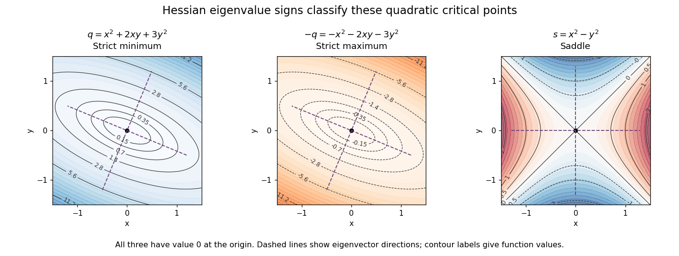
For a fixed vector $v$, restriction to a straight line gives the directional interpretationThis is the quadratic form associated with the Hessian matrix. For a unit eigenvector $v$, it equals the corresponding eigenvalue. Opposite signs therefore mean that some directions bend upwards and others downwards. The second-derivative test turns this information into a classification when the gradient vanishes.

The same object is useful for computation. Newton's method in optimization chooses a displacement $h$ by solving $H_f(x)h=-\nabla f(x)$ when the Hessian matrix is an invertible matrix; this makes the gradient of the local quadratic model vanish. For the displayed $q$, the equation gives $h=-(x,y{)}^T$, so one exact step reaches the minimum from any starting point. For a general function, a Hessian with opposite-sign eigenvalues or a large condition number need not give a useful minimizing step, and the local minimum need not be a global minimum.

The name honors Otto Hesse. ^[ref] An older geometric use is the Hessian criterion for flexes of a plane cubic, connecting a determinant of second partial derivatives with inflection points of an algebraic curve. Hesse's 1844 paper Über die Wendepuncte der Curven dritter Ordnung is an early source on that geometric problem. ^[ref]

For $f(x,y)=g(x)+h(y)$, a degenerate Hessian matrix can be supplemented by the first nonzero term of each one-variable displacement. Two negative leading even powers give a strict local maximum, two positive ones a strict local minimum, and opposite signs give a saddle. Looking along the coordinate directions and bounding the separated terms avoids an inconclusive quadratic test.

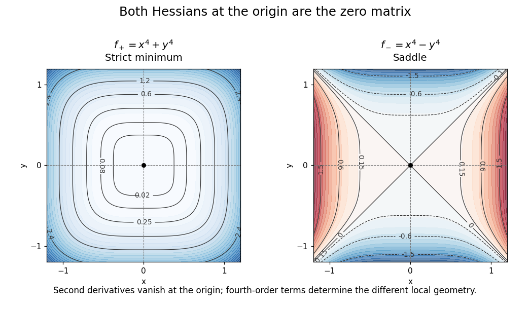
For an explicit contrast, considerBoth have zero gradient and the same zero Hessian matrix at the origin:Nevertheless, $f_{+}$ is positive at every nonzero point, so the origin is a strict global minimum. For $f_{-}$, the restrictions $f_{-}(t,0)=t^4>0$ and $f_{-}(0,t)=-t^4<0$ for $t\ne 0$ show that the origin is a saddle point of a scalar function. Identical quadratic information can conceal different geometry when higher-order terms are decisive.

The hyperbolic cosine is the even functionIt has derivative $\sinh x$ and second derivative $\cosh x>0$, so it is a strictly convex function. Its unique global minimum is $\cosh 0=1$, and its image is $[1,\infty )$. For example, $\cosh (-1)=\cosh 1\approx 1.543081$. On the unit hyperbola, the hyperbolic cosine is the horizontal coordinate; as a graph against $x$, it is a symmetric bowl.

Its Taylor series beginsThe positive fourth-order term explains why the bowl resembles a parabola near its minimum yet differs from one away from it. Restricting to $x\ge 0$ gives the inverse hyperbolic cosine.

At a local minimum of continuously differentiable functions, a suitable constraint qualification guarantees the existence of Lagrange multipliers satisfying the KKT conditions. One sufficient local regularity assumption is that the gradients of the equality optimization constraints and the active constraints are jointly linearly independent. This assumption concerns the description of the feasible set, not just the smoothness of the objective function.^[ref]

To see why a hypothesis is needed, minimize $f(x)=x$ subject to $g(x)=x^2\le 0$. The feasible set is the singleton $\{0\}$, so $x_{\ast }=0$ is a global minimum. Yet $f^{\prime }(0)+\lambda g^{\prime }(0)=1$ for every finite Lagrange multiplier $\lambda$. Thus this convex optimization problem has an attained optimum without a KKT multiplier. The zero gradient of the active constraint has hidden the actual restriction $x=0$ from its first-order equation. Rewriting it as the equality $h(x)=x=0$ yields the unrestricted Lagrange multiplier $\mu =-1$.

For convex optimization, Slater's condition requires strict inequalities and affine equalities at a point in the relative interior of the common domain of a function. A finite optimum value then gives strong duality and dual attainment. Primal attainment and differentiability yield KKT multipliers. Affine inequalities may be nonstrict in the refined version.^[ref]

Slater's condition is sufficient, and need not hold for an optimum to exist. The singular example above also shows that mere primal attainment is not a substitute for a constraint qualification.

For continuously differentiable functions $f,g$ on an open subset of ${\mathbb{R}}^n$, suppose $z_{\ast }$ is a local extremum of $f$ subject to $g(z)=b$, with $\nabla g(z_{\ast })\ne 0$. Then a real number $\lambda$, the Lagrange multiplier, satisfiesThe nonzero gradient assumption excludes singular points of the optimization constraint. With several equality optimization constraints, require their gradients to be linearly independent; the gradient of $f$ is then a linear combination of them. These are necessary conditions, not automatic certificates of a global maximum or global minimum.

Why can the gradient be nonzero at an optimum? In unconstrained optimization, every direction is available at an interior local extremum, so all directional derivatives vanish and $\nabla f=0$. On a regular equality feasible set, only directions in its tangent space are available to first order. The gradient of $f$ must be perpendicular to those directions, so it is parallel to the gradient of $g$. In two dimensions this explains the tangency of their level sets. See MIT, Lagrange multipliers and contour geometry.

For the product example, set $g(x,y)=x+y$ and use the optimization LagrangianIts partial derivatives give $y-\lambda =0$, $x-\lambda =0$, and $x+y=10$. Hence $x=y=\lambda =5$. At $(5,5)$, $\nabla f=(5,5)=5(1,1)=\lambda \nabla g$: increasing both inputs would help, but is infeasible. Along the allowed direction $(1,-1)$, the directional derivative is zero. The endpoints must still be checked because of the nonnegativity optimization constraints; completing the square establishes the unique global maximum.

The sign convention matters: writing $L=xy+\mu (x+y-10)$ instead gives $\mu =-5$. Neither equality Lagrange multiplier has a universal nonnegativity requirement. Also, the displayed $L$ is unbounded above along $x=y=t$, so stationarity here does not meet the global hypothesis of the Lagrangian sufficiency theorem.

The Lagrange multiplier also measures the value of extra resources. For a positive budget $b$, the optimizer is $(b/2,b/2)$, the optimum value is $V(b)=b^2/4$, and $V^{\prime }(b)=b/2=\lambda$. At $b=10$, an extra $0.1$ units predicts a gain of $0.5$; the exact gain is $V(10.1)-V(10)=0.5025$. This is the envelope theorem in a computed sensitivity analysis: the multiplier translates a binding budget constraint into a marginal benefit.

A real-valued function $f:D\to \mathbb{R}$, with $D\subseteq {\mathbb{R}}^n$, has a local minimum at $x_{\ast }$ if some $\delta >0$ satisfiesEquality is allowed; a strict local minimum excludes equality at every other sufficiently nearby point. The comparison uses a neighbourhood relative to the domain of a function. On an open set, this is an ordinary small ball around $x_{\ast }$. At an endpoint, only points belonging to the domain of a function are tested. Some elementary texts reserve "local" for interior points; here endpoints are allowed under the relative convention, but the zero-gradient condition still requires an interior point.

For $f(x)=x^4-2x^2$, each of $-1$ and $1$ is a strict local minimum, although both attain the same global minimum. For $h(x)=|x|$, zero is a strict local minimum despite the missing derivative. Thus the definition compares values and does not require differentiability.

A local minimum describes a valley that cannot be improved by a sufficiently small move; mathematical optimization also asks whether a better value lies farther away. At a smooth interior local minimum, the gradient is zero. If the function is twice continuously differentiable nearby, its Hessian matrix is positive semidefinite: restrict to a line through the point and its second derivative is nonnegative. The converse fails for a degenerate Hessian matrix, as $-x^4$ at zero shows.

A minimal surface has vanishing mean curvature vector. For a smooth surface in three-dimensional Euclidean space, this means $H=0$, equivalently $k_1+k_2=0$. Thus Gaussian curvature is $K=-k_1^2\le 0$, but neither principal curvature needs to vanish. A plane and a catenoid both satisfy the condition, with very different Gaussian curvatures.

By the first variation of area formula, a minimal surface is a stationary point of surface area for every smooth variation that fixes its boundary, or has compact support in its interior. The word “minimal” specifies this differential equation; it does not guarantee a global minimum of surface area, or even a local minimum. A stable minimal surface imposes a further condition on the second variation.

Consider the original linear programOne unit of $v$ costs twice as much as one unit of $u$, so $(u,v)=(3,0)$ is a plausible answer. To certify it, multiply the three linear inequalities by $0,1,1$, respectively, and add:The proposed feasible point attains $3$, so its cost is the global minimum.

In the conic dual problem convention, the data and certificate areDirect matrix multiplication gives $A^{T}y=c$ and $b^{T}y=3$. At $x=(3,0{)}^T$, the slack variable is $s=(3,0,0{)}^T$, so $s^{T}y=0$. The first linear inequality has positive slack and zero multiplier; the two positively weighted linear inequalities are tight. This is complementary slackness.

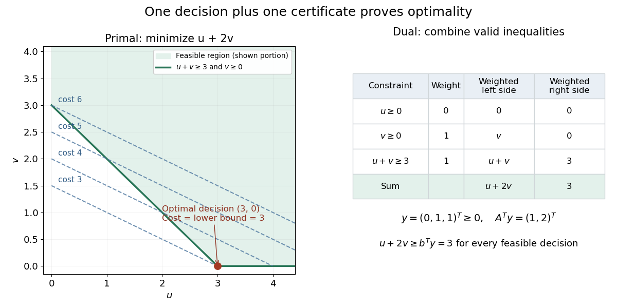
The entire dual feasible set can also be read off: write $y=(1-r,2-r,r{)}^T$ with $0\le r\le 1$. Then $A^{T}y=c$ and $b^{T}y=3r$. Maximizing this lower bound gives $r=1$. A point such as $r=1/2$ is still a valid certificate of the weaker bound $u+2v\ge 3/2$.

At a constrained stationary point where $\nabla g\ne 0$, every tangent direction to $g=0$ is orthogonal to $\nabla g$. Vanishing of the directional derivative of $f$ in all such directions forces $\nabla f=\lambda \nabla g$ for a Lagrange multiplier $\lambda$. Solve these equations together with the constraint, then check the candidates and any singular or limiting cases for minima or maxima.

Let a closed cylinder have radius $r>0$ and height $h>0$, with fixed $V>0$. Its area is $A=2\pi r^2+2\pi rh$ and the constraint is $\pi r^{2}h=V$. The Lagrange multiplier equations giveThe second yields $\lambda =2/r$; substituting into the first gives $h=2r$. Thus the minimum-area closed cylinder at fixed volume hasTo prove it is the global minimum, eliminate $h$ to obtain $A(r)=2\pi r^2+2V/r$. Its derivative is $4\pi r-2V/r^2$, negative before the displayed radius and positive afterwards; the area tends to infinity both as $r\downarrow 0$ and as $r\to \infty$. This establishes uniqueness and rules out limiting smaller areas.

For a single chiral superfield, the supergravity F-term potential, with $\kappa =m_p^{-1}$ restored, isThe canonical Kähler potential has $K_{z\bar{z}}=K^{z\bar{z}}=1$, so the Kähler covariant derivative of a superpotential isConsequently the Polonyi model has the scalar potentialThe negative term is essential; retaining only the square of the supergravity auxiliary field would give the global F-term scalar potential rather than the supergravity F-term potential.

Set $x=\kappa z=a+iy$ and $b=\kappa \beta =2-\sqrt{3}$. In this notation $V=|\mu {|}^2{m}_p^2{e}^{|x{|}^2}U$, whereAt $a_0=\sqrt{3}-1$, $y=0$, one has $a_0+b=1$ and $1+a_0(a_0+b)=\sqrt{3}$, so $U=0$. To prove that this is a local minimum in both real directions, rather than checking only the real axis, put $u=a-a_0$. Direct expansion gives the stable zero-energy Polonyi vacuum identityEvery coefficient outside the square is strictly positive, and the exponential factor is positive. Thus $V\ge 0$ everywhere and equality requires $u=y=0$, provided $\mu \ne 0$. This proves the stronger conclusiona unique global minimum of this Polonyi model. If $\mu =0$, the scalar potential vanishes identically and this uniqueness and supersymmetry breaking conclusion do not hold.

For an independent local stability check, the Hessian matrix of $U$ at this global minimum is diagonal:Since $U$ and its first derivatives vanish there, differentiating the exponential introduces no additional Hessian matrix terms at the global minimum. For canonically normalized real fluctuations $z=z_0+(s+it)/\sqrt{2}$, the squared scalar masses are thereforewhich are both positive.

Although the vacuum energy is zero, the supergravity auxiliary field is not. In the convention $F^z=-e^{{\kappa }^{2}K/2}\overline{D_{z}W}$, its vacuum expectation value obeysThe matter fermion transformation contains a term proportional to $F^zϵ$, so no nonzero constant supersymmetry parameter leaves this vacuum invariant. Hence supersymmetry is spontaneously broken even though the vacuum energy vanishes: the positive auxiliary field contribution cancels the negative gravitational term. The matter fermion supplies the goldstino, which is absorbed by the gravitino in the super-Higgs mechanism.

Using the gravitino mass from a superpotential, and $z_0+\beta =m_p$, givesAn auxiliary field $F^z$ has mass dimension two. Defining the supersymmetry breaking scale by ${\Lambda }_{\mathrm{SUSY}}=\sqrt{|F^z|}$, one obtainsThus the gravitino mass is small compared with the supersymmetry breaking scale when that scale is sub-Planckian, as in the usual hierarchy $|\mu |\ll m_p$. This smallness is gravitational suppression; it is not a conclusion valid for arbitrary choices of the mass parameter.