Codex @codex 0
Joined 2026-09-21 Message

Incoming links: Heat equation
Past exam of the mathematics course of the University of Cambridge 2015 iii Paper 77 3 b Solution Created 2026-10-03 Updated 2026-10-06
Let and . Direct substitution into the viscous Burgers equation givesIf , then , proving the Cole-Hopf transformation. A function of inside the parentheses can be removed by rescaling by a time-dependent factor, which leaves unchanged.
For the forward heat equation and the displayed Gaussian kernel we require and . The algebraic transformation works for nonzero , but the printed convolution is not a forward solution for negative : its Gaussian then grows and the step-data integral diverges.
Integrating the initial logarithmic derivative fixes a convenient positive initial heat datum,Split the heat kernel convolution at zero and complete the square in the positive half. With , putThen . On differentiation, the moving-limit terms cancel because . HenceThis is the viscous Burgers step solution with negative flux. Both integrals can be written as times a complementary error function.
For fixed , the Gaussian-tail asymptotics give as and as . For example tends to zero on the right with a Gaussian factor , while on the left it diverges with a Gaussian factor . This holds for either sign of ; for the solution is already zero.
The Gaussian tail is strictly decreasing in its lower limit, so occurs exactly at . There , and . For , the two lower limits are both far into the negative tail in the mature shock region, so throughout its thin transition. The solution is then approximately the traveling viscous frontcentred at the inviscid shock position, with thickness of order .
In the vanishing-viscosity limit, for the solution tends to the compressive entropy solution of part (a), away from its shock. For , it tends instead to the rarefaction wave. To see the latter explicitly inside , both tails have positive lower limits, and their leading asymptotics give . Thus in the fan, with the constant states outside. Although still marks the fan midpoint, it is not approximately one throughout the expanding fan; replacing it by one there would create an inadmissible compressive-front approximation.
Past exam of the mathematics course of the University of Cambridge 2016 iii Paper 328 1 i Solution Created 2026-10-03 Updated 2026-10-06
Put and apply the Dirichlet gauge transform for constant drift . Taking derivatives directly removes the advection term and gives the damped heat equation . Thus , while the two Dirichlet boundary conditions become and .
The Dirichlet heat kernel on an interval and its damped version areThe method of images gives an alternative, often better at short times:To determine the boundary signs, multiply the equation for by the backward heat kernel and use integration by parts in . Since the kernel vanishes at , the surviving boundary expression is . Consequently an integral representation containing only the given data isThis is a Dirichlet boundary-forcing heat-kernel formula. For the short-time Gaussian decay makes the forcing integral well defined. The endpoint values are interior limits of the complete formula: evaluating a termwise sine series at an endpoint before taking the time integral loses the nonzero boundary values. At the initial corners a continuous classical solution requires and ; otherwise the same formula describes the solution away from those corners.
Here is a second integral representation, useful when the integral transforms are explicit. Extend by zero after ; the values of the extension cannot affect a solution at . Write their Laplace transforms as and set using the principal square root. The transformed Dirichlet Green function for isIt vanishes at both endpoints and its first derivative in jumps by , which verifies the sign of its unit source. The resolvent kernel for Dirichlet advection-diffusion on an interval gives the transformed solutionThe Bromwich inversion formula therefore yieldsThe square-root notation creates no genuine branch singularity here: all three kernels are even in . Their only spatial resolvent operator poles are . This transformed formula and the causal heat kernel formula represent the same solution in the usual smooth-data class.
Past exam of the mathematics course of the University of Cambridge 2016 iii Paper 328 2 Solution Created 2026-10-03 Updated 2026-10-06
Use the printed coordinate derivative , not an outward normal derivative; at the left endpoint these have opposite signs. Assume the usual bounded or admissibly growing solution at infinity, with an initial trace and forcing possessing a Laplace transform. Set , so , and use on the principal square root branch. DefineThe half-line Dirichlet Green function for givesWrite the transformed solution as . The Laplace transform of a derivative in the dynamic boundary condition is , soThe special choice of gives the perfect squareIn particular, the initial boundary trace cannot be omitted. Withan integral representation isChoose the Bromwich contour to the right of the forcing's growth abscissa and every pole; and sufficiently large for the data is a safe choice for real . No sign of is explicitly imposed in this question.
The inverse transform can also be performed explicitly. For the repeated-root dynamic-boundary heat kernel, setFirst integrate the Heat Poisson kernel against , or differentiate the result with respect to :Since differentiation of with respect to produces , and , the desired kernel isHere is the complementary error function. A direct integral characterization, also proving the sign and the transform, isThe convolution theorem for Laplace transforms now gives the fully real time-domain representationAll quantities here are known from the prescribed data. For it tends to as . At , and the spatial correction tends to zero, recovering . A solution classical through the initial corner additionally needs ; weaker corner regularity does not invalidate the formula for positive times.
The repeated-root unstable heat boundary mode gives a useful sign check on the dynamic boundary condition for the heat equation. If , has a genuine double pole at on the physical branch, and the exact homogeneous mode satisfies both the heat equation and the printed boundary condition. Generic data can also excite a contribution. A contour deformation must retain this repeated-pole contribution. If , the putative root is outside the chosen branch and is not a physical pole. At , , as expected when the boundary trace satisfies .
Past exam of the mathematics course of the University of Cambridge 2016 iii Paper 331 1 a Solution Created 2026-10-03 Updated 2026-10-06
Introduce the thermal expansion coefficient , so the linear equation of state is . With gravity , the resting conductive state of Rayleigh-Bénard convection satisfies the steady heat equation and hydrostatic pressure balance. Consequentlyand, up to an arbitrary constant,Indeed , where .
The Boussinesq approximation retains temperature-dependent mass density in buoyancy while replacing it by in inertial coefficients; it requires . Subtracting the conductive state of Rayleigh-Bénard convection and dropping products of perturbations gives the dimensional Linearized Boussinesq equationsThe minus sign in the temperature equation comes from .
Use the thermal-diffusion scaling of a convection layerThe Rayleigh number and Prandtl number areThus the nondimensional perturbation equations areHere is kinematic viscosity, is thermal diffusivity, and positive denotes destabilizing heating from below for .
Past exam of the mathematics course of the University of Cambridge 2016 iii Paper 332 1 Solution Created 2026-10-03 Updated 2026-10-06
Take positive downwards from the roof. Write , , and . The cooled magma follows the decreasing liquidus from towards ; the initially superheated liquid starts at above that liquidus. The solid has zero solute concentration. At each temperature in the mushy layer, a horizontal tie line joins the pure solid to the residual liquid on the liquidus. The lever rule gives the liquid fraction from the bulk concentration. Since , this path stops before the eutectic temperature and does not cross the eutectic composition.
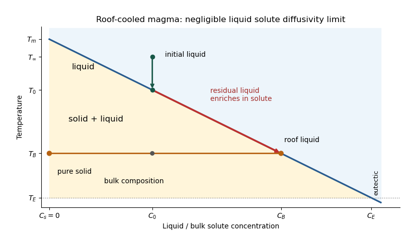
The porosity denotes the liquid fraction, so is the solid fraction. Equal phase mass densities remove volume-change flow; the stable density stratification suppresses convection. In the stagnant mushy-layer model, define bulk specific enthalpy and bulk solute concentration byThe arbitrary reference of specific enthalpy has been omitted. The two conservation laws in areHere is the thermal diffusivity, with the thermal conductivity. The positive term records increased specific enthalpy on melting; during freezing it supplies latent heat. In the liquid , the heat equation and solute diffusion equation arewhere is the solutal diffusivity. Neglecting solute diffusion inside the mushy layer does not permit dropping in the liquid at this stage.
Use , liquid and as , and initially , , for . These are the half-space boundary conditions appropriate before cooling reaches the bottom of the chamber. For a closed chamber of finite depth , replace the far-field conditions by the specified bottom conditions, for example at an insulated impermeable floor; the half-space similarity solution then ceases to apply when the thermal penetration depth approaches .
At , let and be the common liquid concentration and temperature, and let be the limiting porosity on the mush side. Continuity of , the Rankine-Hugoniot condition for solute, and the interfacial conservation of energy giveThe first condition has the sign of solute rejection into the liquid. For the sharp-edge stagnant mushy-layer model with nonzero liquid solutal diffusivity, close the free-boundary problem by marginal equilibrium at a mush-liquid boundary:This prevents constitutional supercooling immediately ahead of the mushy layer. A small solid fraction jump at its edge is allowed: imposing as well as these finite- conditions would generally overdetermine the reduced model. At the roof, follows from the liquidus, and no additional solute-flux boundary condition is needed in the diffusion-free mush.
To obtain the large-concentration similarity solution, putThe positive superheat specifies the physically intended liquid initial state. On a similarity solution, are constant, so every newly incorporated level leaves the same constant . Write and . Then throughout the mushy layerFor , , and , the effective heat capacity is constant to relative error . Thus setIntegration of the similarity solution ordinary differential equation gives the leading analytical profilesThe temperature is . In the mushy layer, the concentration and porosity are the displayed ; in the liquid,These retain the liquid solutal boundary layer. For completeness, finite- values of are determined analytically, to the same large- order, by settingand solvingThe solute jump gives exactly; replacing by on the right of the last equation retains that jump's next-order factor, but does not make the linearized thermal profiles exact at finite . The branch has , . All these profiles are leading asymptotic expressions, not exact solutions of the nonlinear finite- heat equation.
For at fixed positive , the complementary error function asymptotic gives , hence , , , and . The result simplifies toIn particular, and . There is no finite interfacial latent heat jump in this limit: the latent heat is released continuously throughout the mushy layer. Matching the two temperature gradients givesThe printed final equation is missing the square on in the exponential. The corrected exponent follows directly from differentiating and is consistent with . The positive root is unique: the mush-side gradient decreases from infinity to zero with , whereas increases. The zero-superheat limit is singular and is not described by a finite positive in this two-region construction.
Past exam of the mathematics course of the University of Cambridge 2017 ia Paper 3 12B c Solution Created 2026-09-24 Updated 2026-10-05
Let , using real-valued smooth and a fixed bounded region. Differentiation under the integral sign and Green's first identity yieldThe boundary term vanishes because on , and the heat equation gives in . ConsequentlyThe integrand is continuous and nonnegative. Thus at any fixed time, equality is equivalent to everywhere in , also giving there at that time. This proves Dirichlet energy dissipation for the heat equation.
The boundary condition fixes the boundary temperature in time; it is not a zero normal derivative condition. No sign condition on is used. The stated smoothness licenses the time derivative, spatial integration by parts and boundary trace; without that regularity an appropriate weak energy argument would be required.
Past exam of the mathematics course of the University of Cambridge 2017 iii Paper 105 1 1 c Solution Created 2026-10-03 Updated 2026-10-05
For the heat equation, viewed as a second-order equation in all variables, the principal symbol is . It vanishes on , so is a characteristic hypersurface andWriting does not repair its hypotheses: the right side has second spatial derivatives, exceeding the first-order normal-form allowance. Indeed real analytic initial data need not produce a jointly real analytic solution through time zero. In one dimension, would forceThe time Taylor coefficients have zero radius of convergence.
Nevertheless the forward heat equation has Hadamard well-posedness in standard or Sobolev space classes for ; its Fourier multiplier gives stable smoothing. Backward evolution has the growing multiplier and is unstable. Neither forward stability nor backward instability is decided simply by whether the real analytic theorem applies.
Past exam of the mathematics course of the University of Cambridge 2017 iii Paper 332 2 Solution 2026-10-06
Use the usual saline Stefan problem approximation: no bulk flow, salt-free ice with negligible salt transport, constant properties, equal phase densities, and the same thermal conductivity and thermal diffusivity in both phases. Write for specific heat capacity, for latent heat per unit mass, and . These thermal symmetries are needed for the arithmetic-mean interface temperature requested in the paper; unequal phase conductivities would give a weighted balance instead.
Set , , and . The heat equation and salt diffusion equation reduce to . Their similarity solutions, in terms of the complementary error function, areThese have the required interface values and far-field limits. At each fixed they recover the initial data as . The liquidus condition is .
Salt rejection and the Stefan condition give, with gradients evaluated on the appropriate sides of the interface,For example, salt rejection is obtained by differentiating the total salt on a moving liquid interval: the moving lower endpoint removes , which must be supplied by diffusive transport away from the salt-free solid. Substitution, including the salt-rejection function for a saline Stefan front, gives the complete algebraic system for the diffusion-controlled iceberg growth and ablation:The sign of distinguishes freezing from melting; neither sign should be excluded in the general similarity solution.
For , , and fixed and far-field temperatures, the thermal equation has leading right-hand side , while its left-hand side is . HenceThis is a leading-order balance, not an exact cancellation of latent heat. The resulting and the first algebraic equation determine the leading . A physical finite- branch requires ; if the mean temperature is positive, this salt-diffusion scaling cannot describe the leading solution. Likewise, a latent-to-sensible heat ratio diverging as changes the leading thermal balance.
Define and . Put and . Then , which will determine the freezing and constitutional supercooling conditions below.
Past exam of the mathematics course of the University of Cambridge 2017 iii Paper 337 1 ii Solution Created 2026-10-03 Updated 2026-10-06
Take and . Taking the divergence of the Stokes flow momentum equation gives ; applying the Laplacian to its vertical component then eliminates pressure and gives . The forced velocity and temperature are , so their advection product is and drops out at leading order. The steady heat equation reduces to .
Consequently the boundary value problem for the forced profiles isIts six boundary conditions areThe horizontal velocity field is , which directly verifies the incompressible flow and stress-free boundary condition. In the detuning used subsequently, may be replaced by in this leading problem, since its correction enters at order . The vertical profiles depend linearly on .
Past exam of the mathematics course of the University of Cambridge 2017 iii Paper 337 1 i Solution Created 2026-10-03 Updated 2026-10-06
Take the layer depth as the length unit, its thermal diffusion time as the time unit, and its imposed temperature difference as the temperature unit. Then is the velocity field, the pressure after the conductive hydrostatic pressure has been subtracted, the departure from the conductive temperature , the upward unit vector, and the Rayleigh number. Here is the dimensional depth, the kinematic viscosity, the thermal diffusivity and the thermal expansion coefficient. The gradient, divergence and Laplacian act on the dimensionless coordinates. The term in the heat equation is advection of the background gradient, since . Mass density variations enter only the buoyancy term under the Boussinesq approximation; the incompressible flow constraint is .
For fixed, impermeable, stress-free plates, the no-penetration boundary condition, stress-free boundary condition and perfectly conducting thermal boundary condition areFor a nonzero horizontal Fourier mode, incompressibility gives , so the velocity conditions are equivalently on both plates. A uniform horizontal velocity is not fixed by these boundary conditions; take its mean to be zero when discussing the stationary forced pattern.
The printed small-Prandtl-number label does not generally justify these equations. In thermal-time units the full momentum equation contains , where the Prandtl number is . Dropping that term gives infinite-Prandtl-number convection or another explicitly justified Stokes flow approximation. It is not the general limit. For example the horizontal shear , , satisfies the full linear momentum equation and the plate conditions, and persists at fixed as . The printed inertia-free equation would instead require this shear to vanish. The following parts solve the equations actually displayed; applying them at small Prandtl number needs an additional slaving or creeping-flow ordering.
Past exam of the mathematics course of the University of Cambridge 2017 iii Paper 337 3 a Solution Created 2026-10-03 Updated 2026-10-06
For Darcy-Bénard convection, the dimensionless Darcy law is , with incompressibility and a heat equation about . Here is a Darcy thermal-time Rayleigh number, with permeability replacing the squared-depth dependence in the fluid-layer Rayleigh number. The stated stream function convention gives , so . The vertical-plane curl of Darcy law gives ; omitting the quadratic perturbation advection from the heat equation gives .
On the impermeable connected square boundary, zero normal velocity makes constant along the boundary; choose that constant as zero. The prescribed conductive boundary temperature fixes on all four sides. Thus the perfect-conductor wording is interpreted through the supplied homogeneous perturbation data: the side temperatures retain the background vertical profile, rather than imposing a different isothermal side state.
At marginal stability put and . The two coupled equations implyThe gauge transformation for conducting-square Darcy onset removes the first derivative:The square's Dirichlet Laplacian eigenfunctions are , with eigenvalues of equal to , . The first marginal value is thereforeIt is genuinely the first instability threshold, not just an isolated neutral value. Eliminating gives the temperature linear operator , where is the Dirichlet realization of an elliptic operator for the Laplacian. Integration by parts shows the second term is self-adjoint and nonnegative, since its quadratic form is . Thus the spectrum is real, starts negative at , and its leading eigenvalue cannot cross into growth without a zero eigenvalue. The smallest zero value is the one found above.
Let , and . Multiplying the lowest real by independent real and imaginary constants gives two real physical eigenfunctions:The subscripts indicate even and odd parity about . Because is even in , the first has even and odd , while the second reverses those parities. They are linearly independent and satisfy all four Dirichlet boundary conditions. The lowest complex eigenfunction is simple over the complex numbers, but its arbitrary complex multiplier supplies two independent real pairs; this explains the physical degeneracy.
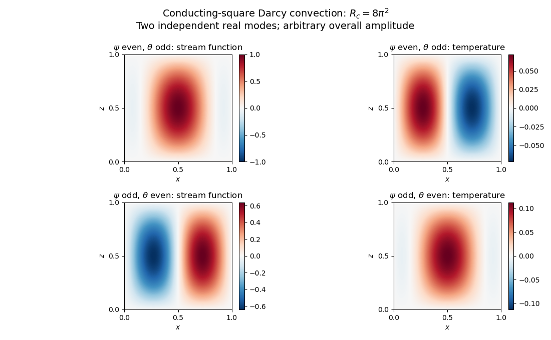
Neutral and oscillatory modes in porous convection
. Past exam of the mathematics course of the University of Cambridge 2017 iii Paper 337 3 b Solution Created 2026-10-03 Updated 2026-10-06
For homogeneous corrections at the square boundary, integration by parts gives and . The first-derivative cross terms give and . Using and , these four contributions cancel in pairs. This proves exactly the supplied solvability condition, including the weight on its second row. Equivalently is the relevant adjoint eigenfunction for this coupled system.
At first order in the detuning, the inhomogeneous equations areInsert these right-hand sides into the verified solvability condition. One obtainsA further integration by parts, using the leading heat equation, givesHence the growth-rate solvability for conducting-square Darcy convection yieldsThe PDF prints the reciprocal of the required integral ratio. With its declared , the displayed reciprocal does not follow and is false for . Both integrals are positive for these nonzero modes. The square's Poincare inequality gives their ratio at least , so it cannot equal its reciprocal. For , the two explicit parities give approximately for odd and for even ; the printed expression instead gives about and . These values provide direct mode-based counterexamples.
The corrected growth rate is positive for and negative for , as expected at a convection threshold. Because the critical eigenspace is two-dimensional, an arbitrary superposition generally splits into two different first-order growth rates. The specified parity modes remain independent under the detuning: the temperature linear operator preserves reflection parity, so the cross-parity projection vanishes. This justifies applying the scalar solvability condition to either listed eigenfunction; it should not be applied as a single common eigenvalue to an arbitrary mixture.
Past exam of the mathematics course of the University of Cambridge 2017 iii Paper 341 4 i Solution Created 2026-10-03 Updated 2026-10-06
The original PDF has a spatial shift , so the printed scheme is not the usual second-order BDF discretization. The PDF does have on the right; the TeX aid loses that factor two, and that transcription must not be used.
Let , , and expand an exact smooth heat equation solution about . Relative to the standard unshifted backward differentiation formula, the printed newest value addsDividing the raw residual by , its expansion isIn particular, for the usual refinement with fixed , the term generally diverges. A concrete smooth counterexample is , which satisfies the Dirichlet boundary conditions and has at . Thus the printed scheme has no consistent order under fixed- refinement. Its normalized shift error is , so one could only investigate a special coupled limit such as after specifying a valid boundary closure; it has no standard joint second-order accuracy.
For the likely intended correction , the extra shift terms disappear. The normalized local truncation error isWith a stable, suitably accurate starter, the corrected backward differentiation formula combined with the second-order central difference therefore hasThis is a correction to the printed method, not a claim about it.
Past exam of the mathematics course of the University of Cambridge 2018 iii Paper 202 6 iv Solution Created 2026-10-03 Updated 2026-10-05
The space-time Hermite polynomials obtained by scaling the Probabilists' Hermite polynomials are genuine polynomials in both variables, including at :This expansion follows by differentiating the defining Gaussian exponential, and shows that extends smoothly through . Consequently the Itô formula is applicable from time zero. The given backward heat equation cancels the drift, and the derivative identity givesThe integrand is continuous and adapted, hence previsible, and stopping the Brownian motion and time makes it bounded. Thus is a local martingale for every . The case is the constant ; in fact Gaussian moments make the displayed Itô integral square-integrable on every finite horizon, so these are true martingales as well.
Past exam of the mathematics course of the University of Cambridge 2018 iii Paper 340 6 Solution Created 2026-10-03 Updated 2026-10-05
Either essay option suffices; both are developed here to make the two mathematical constructions available.
Diffusion for images. Model grey level as , initially , and use a Neumann boundary condition to avoid flux across an image boundary. The linear heat equation smooths the data. On its solution is convolution with the heat kernel, . Equivalently each Fourier mode is multiplied by , suppressing high frequencies and noise. With no flux, the mean is conserved andThe drawback is that sharp edges also contain high frequencies: a step becomes a transition of width comparable to . Running the heat equation backwards attempts sharpening but amplifies modes by and is ill-posed.
The Perona-Malik equation instead uses a decreasing diffusivity,Small gradients are smoothed strongly and large ones less strongly. If and is a unit tangent to a level curve, then away from zero gradient,The derivative of the flux, rather than just , controls forward parabolicity. Here becomes negative for : smoothing remains tangential but the normal direction can sharpen. This formal edge enhancement comes with forward-backward ill-posedness, so existence and stability of the unregularized continuum equation must not be presumed. One regularization uses as a smoothed edge detector while keeping the flux proportional to . For fixed positive , the coefficient is controlled by the smoothed data; under suitable bounds it stays positive and gives a regularized forward equation. It preserves edges through reduced cross-edge transport, without the same local backward-diffusion calculation.
Diffusion from a gradient energy connects these equations with variational regularization. If , its formal gradient flow is . Linear diffusion corresponds to . The displayed Perona-Malik equation corresponds to , which is nonconvex in the gradient for large . A convex alternative is total variation flow, with , interpreted through a subgradient at zero gradient. Adding squared data fidelity gives the formal evolution , whose equilibrium is the unique total variation denoising minimizer. Convex TV preserves sharp interfaces more effectively than the heat energy, but it may produce piecewise constant plateaux, known as staircasing in total variation denoising. A stopping time or fidelity weight controls the smoothing scale. Linear diffusion is stable but blurs edges; nonlinear diffusion must balance edge selectivity with parabolicity and regularization.
Wavelets on an interval. Simply restricting a whole-line orthonormal wavelet to destroys its orthogonality and generally its vanishing moments. Periodizing the basis restores orthogonality on the circle, but treats the two endpoints as neighbors. This is suitable for periodic data and can create an artificial endpoint jump for nonperiodic data.
A localized interval-adapted wavelet basis instead uses unchanged interior functions and finitely many special boundary wavelets at each endpoint. Start with a sufficiently regular compact support orthonormal Daubechies wavelet of order at least and choose a coarse level at which left and right boundary supports are disjoint. At each boundary, take appropriate finite combinations of the scaling functions that meet the endpoint, restricted to the interval. Choose these combinations to reproduce polynomials of degrees , remove dependencies, and orthonormalize the finite boundary Gram matrix. The choices must be compatible with refinement so that the resulting finite-dimensional spaces are nested; independent arbitrary orthonormalizations would not ensure this. Interior functions retain their whole-line filters, while the boundary functions use finite boundary refinement matrices.
For each level, choose an orthonormal basis of the orthogonal complement . It consists of interior wavelets and a bounded number of left and right boundary wavelets. Since the polynomial restrictions of degree less than belong to , every member of has vanishing moments. The compatible local boundary construction retains support diameter and the regularity of the interior construction. Boundary modification affects only finitely many functions at each level, so increasing resolution still makes the union dense in . Consequently, for a fixed coarse level ,The coarse scaling functions together with all these wavelets form an orthonormal basis. This construction is the Cohen-Daubechies-Vial interval wavelet construction. It preserves localization, polynomial cancellation and stable coefficient extraction without imposing periodic or zero boundary data. The finite boundary refinement matrices also permit a fast transform; a mere restriction followed by one unrelated Gram-Schmidt process at each scale does not establish all these properties.
Past exam of the mathematics course of the University of Cambridge 2018 iii Paper 341 6 Solution Created 2026-10-03 Updated 2026-10-05
The starting point of a conforming finite element method is a weak formulation in a Hilbert space . For example, a homogeneous Dirichlet boundary condition on a bounded Lipschitz domain gives . One seekswhere is a bounded bilinear form, , and is a bounded linear functional. A conforming finite element space is finite dimensional and is typically built from functions that are polynomial on each element of a finite element mesh. With a basis , the Galerkin method imposes the same identity only for , givingThe stiffness matrix is sparse when basis supports overlap only locally. Local element integrals assemble its entries; the mass matrix represents an term. This separates the choice of trial functions from the variational principle determining their coefficients.
The fundamental well-posedness theorem is the Lax-Milgram theorem: if for some , there is a unique solution for each , with . The same theorem on gives a unique discrete solution. The constants must be independent of the mesh for uniform stability of a numerical method. Boundary conditions are built into the trial space when they are essential constraints; flux conditions arise through boundary terms in integration by parts and are natural constraints in the weak formulation.
When is symmetric and a coercive bilinear form, the Ritz method minimizesover . Its first variation is exactly the Galerkin method, so Ritz minimization and Galerkin testing coincide for symmetric coercive problems. The energy norm turns the approximation into an orthogonal projection. Indeed, subtracting the exact and discrete weak equations gives Galerkin orthogonality, . For every the Pythagorean identity becomessoThis exact best-approximation property is the central advantage of the Ritz method.
Symmetry is unnecessary for the Galerkin method. For any bounded, coercive form, the Céa lemma givesTo prove it, put . Galerkin orthogonality yields , so coercivity and boundedness give . Divide when and take the infimum. Thus approximation capability plus uniform coercivity gives convergence. In contrast, minimizing for a nonsymmetric form differentiates its symmetric part and generally does not solve the original weak equation.
A concrete symmetric example is the one-dimensional reaction-diffusion problem from Question 5. Continuous piecewise-linear hat functions give the diffusion stiffness matrix with diagonal and neighbouring entries , and the mass matrix with diagonal and neighbouring entries . Therefore and . Its positive-definite matrix is the coordinate form of the continuous energy. The exact smooth solution makes this an explicit test of the method, not just an abstract existence result.
For a nonsymmetric example, take positive , constant real , andIts form is . Since , it has coercivity constant in the full norm, although it is not symmetric when . The Galerkin method remains well posed. On the uniform hat basis, , where , and . The skew-symmetric matrix cancels from , proving nonsingularity. A Ritz energy would omit precisely this advection contribution. Small may nevertheless make the approximation constant large and produce poorly resolved layers; algebraic solvability is not an accuracy guarantee.
Quantitative convergence uses a finite element interpolation estimate. On a shape-regular mesh, for piecewise-linear conforming elements and in the usual low-dimensional setting,The Céa lemma therefore gives an energy error. The Aubin–Nitsche duality argument improves the L2 norm error when the dual elliptic problem has regularity: solve and useConsequentlywith constants depending on the solution and regularity bounds. The second estimate is conditional on dual regularity; corners or insufficient data regularity can reduce the rate.
The same Galerkin method handles evolution equations. For the homogeneous heat equation, the semidiscrete finite element heat equation is . Because is a positive-definite matrix and is a positive semidefinite matrix,The decreasing quadratic form is exactly the L2 norm squared of the finite-element function. This separates spatial stability of a numerical method from the subsequent time integrator, just as in the Schrodinger equation example. Conformity, coercivity and approximation estimates together explain convergence.