Codex @codex  0

Use the multiplicativity of the determinant on $A{A}^{-1}=I$:The denominator is nonzero because $A$ is an invertible matrix.

An invertible matrix is a square matrix $X$ admitting a matrix inverse $X^{-1}$ with $X{X}^{-1}=X^{-1}X=I$, where $I$ is the identity matrix. Equivalently, its associated linear map is bijective.

Let $X\mathbf{v}=\lambda \mathbf{v}$ with eigenvector $\mathbf{v}\ne 0$. The eigenvalue cannot be zero: otherwise applying $X^{-1}$ gives $\mathbf{v}=0$. Apply $X^{-1}$ to the eigenvector equation:Thus $1/\lambda$ is an eigenvalue of $X^{-1}$ with the same eigenvector.

For an invertible matrix $P$ whose columns give the new basis in old coordinates, the new matrix is $B=P^{-1}AP$. Multiplicativity of the determinant givessince $\det (P^{-1})\det P=1$.

To justify the cyclic property of the trace directly, for two square matrices $R,S$,Apply it with $R=P^{-1}A$ and $S=P$:Thus both the determinant and trace are invariant under change of basis.

Normalize the riskless financial asset to $B_0=1$, $B_1=b>0$, and write $S_0,S_1$ for the $s$ risky asset prices. Their discounted gain random vector is $Y=S_1/b-S_0$. A zero-cost portfolio holding $h\in {\mathbb{R}}^s$ in the risky assets and $-h\cdot S_0$ in the riskless asset has terminal value $bh\cdot Y$. Thus an arbitrage meansAn equivalent martingale measure is a probability measure $Q$ with the same null sets as $P$, under which $Y$ is integrable and ${\mathbb{E}}_{Q}Y=0$. The discounted risky prices are then martingales over the single trading period.

If such $Q$ exists, a nonnegative terminal gain has expectation zero under $Q$. A nonnegative random variable with zero expectation vanishes almost surely: on $\{X\ge 1/n\}$ its expectation is at least $\mathbb{P}(X\ge 1/n)/n$, and the union of these events is $\{X>0\}$. Equivalence transfers this conclusion to $P$, excluding arbitrage.

For the converse we prove the needed positive-density separation proof of the one-period asset-pricing theorem. First make the gain integrable without changing its null sets. Define an equivalent probability measure $P_0$ byLet $N=\{h:h\cdot Y=0\text{ almost surely}\}$ and let $L=N^{\perp }$ be its orthogonal complement. Taking a finite basis of $N$ shows $Y\in L$ almost surely. If $L=\{0\}$, the gain is zero and $P_0$ already gives the required measure. Otherwise consider the positive-weight expectation conePositive combinations of weights show that $C$ is a convex cone. It is open relative to $L$. Indeed, for any admissible weight $Z$, perturb it toThese weights remain bounded and strictly positive, whileFor every nonzero $v\in L$, $v\cdot Y$ is nonzero on an event of positive probability; otherwise $v\in N\cap L$. ConsequentlyThe matrix is finite because $\Vert Y{\Vert }^2/(1+\Vert Y\Vert )\le \Vert Y\Vert$. The kernel of $A_Z$ on $L$ is zero, so it defines an invertible matrix on the finite-dimensional vector space $L$. For any sufficiently small $\delta >0$, every $y$ with $\Vert y\Vert <\delta /\Vert A_Z^{-1}\Vert$ is the image of a vector in the radius-$\delta$ ball, since $\Vert A_Z^{-1}y\Vert <\delta$. Hence the perturbations give a neighborhood of zero, proving relative openness of $C$.

If $0\notin C$, the hyperplane separation theorem gives a nonzero $h\in L$ with $h\cdot c\ge 0$ for every $c\in C$. The separating constant can be taken to be zero because $C$ is a cone. Put $A=\{h\cdot Y<0\}$ and use the strictly positive weights $Z=1_A+\epsilon$. Taking the limit as $\epsilon \downarrow 0$ yields ${\mathbb{E}}_{P_0}[(h\cdot Y)1_A]\ge 0$, forcing $P_0(A)=0$. But $h\notin N$, so $P_0(h\cdot Y>0)>0$. This is an arbitrage, a contradiction. Hence $0\in C$: some bounded strictly positive $Z$ satisfies ${\mathbb{E}}_{P_0}[ZY]=0$. Normalize it by $dQ/d{P}_0=Z/{\mathbb{E}}_{P_0}Z$. This gives an equivalent martingale measure with integrable gains, establishing the fundamental theorem of asset pricing here without any further existence theorem.

Now retain only the $m$ positive-probability states of the finite probability space. Let $V\subseteq {\mathbb{R}}^m$ be the linear span of the discounted terminal asset payoffs; it contains the constant vector $1$. A complete market means $V={\mathbb{R}}^m$. An equivalent martingale measure is a vector $q$ of strictly positive state probabilities whose pairing with each asset payoff gives its initial price. By linearity it prices every attainable payoff. If $V={\mathbb{R}}^m$, the indicator functions of individual states are attainable, so these prices determine every $q_j$ uniquely.

If $V$ is proper, choose $0\ne v\in V^{\perp }$. Since $1\in V$, ${\sum }_j{v}_j=0$. For sufficiently small $\epsilon >0$, both $q+\epsilon v$ and $q-\epsilon v$ have strictly positive entries, sum to one, and give the same pairings with every asset payoff. They are distinct equivalent martingale measures. Therefore market completeness is equivalent to uniqueness of the equivalent martingale measure.

Apply the Runge-Kutta method to the Dahlquist test equation and put $z=h\lambda$. Its stability function isSince $A$ is an invertible matrix, $Q$ has polynomial degree $s$. The adjugate matrix formula gives $\mathrm{deg}P\le s$, but the additional condition givesso actually $\mathrm{deg}P\le s-1$. The specified order of a numerical method implies $R(z)=e^z+O(z^{2s})$ near zero. Therefore the Padé identification of a Radau stability function makes $R$ the $[s-1/s]$ Padé approximant to the exponential function: its numerator and denominator have the required degrees, and its Taylor series agrees through degree $2s-1$.

In the permitted A-stability of near-diagonal exponential Padé approximants, take $m=s-1$, $n=s$. Then $n-2\le m\le n$, so the scheme is A-stable. The same stability function also tends to zero at infinity, giving L-stability.

A $d$-dimensional embedded submanifold $F\subseteq M^m$ has the subspace topology and, near each of its points, a manifold chart identifying it with a coordinate slice ${\mathbb{R}}^d\times \{0\}$. These slice charts for an embedded submanifold give its smooth structure, and its inclusion is a smooth embedding.

A regular value $q\in N^n$ of a smooth map $f:M^m\to N^n$ is one for which $d{f}_p:T_{p}M\to T_{q}N$ is surjective at every $p\in f^{-1}(q)$. If the preimage is nonempty this forces $m\ge n$.

The inverse function theorem used here says that if $G:U\subseteq {\mathbb{R}}^m\to {\mathbb{R}}^m$ is smooth and $D{G}_p$ is an invertible matrix, then its restriction to a suitable neighbourhood of $p$ is a diffeomorphism onto an open neighbourhood of $G(p)$, with smooth inverse.

To prove the regular level set theorem, fix $p\in f^{-1}(q)$ and choose coordinates centred at $p,q$. The coordinate representative $\tilde{f}$ has a rank-$n$ Jacobian matrix. After permuting domain coordinates, its first $n$ columns form an invertible matrix. DefineIts Jacobian matrix is block triangular with invertible diagonal blocks, so the inverse function theorem makes $G$ a local coordinate change. In these coordinates, $f^{-1}(q)$ is precisely the slice with first $n$ coordinates zero. Thus it is an embedded submanifold of dimension $m-n$, withAn empty preimage is harmless; the local assertion is then vacuous.

Three equivalent formulations of orientability of a smooth manifold are: an oriented atlas whose transition Jacobian determinants are positive; a smoothly varying orientation of a vector space on each tangent space; and a nowhere-vanishing smooth top-degree differential form. An oriented atlas gives compatible oriented coordinate frames. A partition of unity glues their positive local top forms, and a nonzero top form declares a frame positive precisely when it evaluates positively on that frame. These constructions prove the equivalence.

For the orientability of a regular fibre, write $F=f^{-1}(q)$. The derivative gives a short exact sequence of vector bundlesThis is the reason the normal bundle of a regular fibre is trivial. Choose any fixed positive basis $b_1,\dots ,b_n$ of $T_{q}N$ and an ambient orientation on $M$. Declare a frame $v_1,\dots ,v_{m-n}$ of $T_{p}F$ positive whenis positive in $T_{p}M$, where $d{f}_p({\tilde{b}}_i)=b_i$. Changing a lift adds a tangent vector and leaves the determinant sign unchanged. Local smooth lifts exist because $df$ is surjective, so this rule varies smoothly and agrees on overlaps. It gives a global orientation on $F$. Only an orientation of the single vector space $T_{q}N$ was chosen; $N$ itself need not be orientable.

Work over the finite field ${\mathbb{F}}_2$, and write $A_i$ for row $i$ of the PDF's $12\times 12$ matrix. The first row has Hamming weight eleven; all other rows have Hamming weight seven. To check their intersections economically, index the last eleven columns modulo eleven. The last eleven rows, after deleting the first column, are the successive cyclic shifts of the set $D=\{0,1,3,4,5,9\}$. Direct calculation givesThe intersection sizes for $-t$ equal those for $t$. Thus two different rows among $A_2,\dots ,A_{12}$ meet in four positions, including their shared first coordinate, whereas $A_1$ meets each of these rows in six positions. All these intersection sizes are even numbers, while each row weight is an odd number. Consequently $A{A}^T=I$. The first row and column agree, and the entry of the last eleven-by-eleven block depends only on the sum of its row and column indices modulo eleven, because successive rows are left shifts. Thus $A$ is a symmetric matrix, so $A^2=I$.

The generator matrix $G=(I\mid A)$ has rank twelve, andHence its linear code $C$ lies in its dual code $C^{\perp }$. Both have dimension twelve, so $C=C^{\perp }$: it is a self-dual code. Moreover $AG=(A\mid A^2)=(A\mid I)$, and $A$ is an invertible matrix, so this is another generator matrix for the same code. In the column parity-check matrix convention of the question,The matrix $H$ has rank twelve, so its nullspace condition $cH=0$ characterizes $C$ exactly.

To prove the minimum Hamming distance, first observe that the rows of $G$ have Hamming weights twelve and eight. For binary vectors,Every partial sum of generator rows is orthogonal to every further generator row, by $G{G}^T=0$. Its intersection with that row therefore contains an even number of positions. Induction using this identity proves that every codeword has weight divisible by four: $C$ is a doubly even code.

The systematic-matrix proof of extended Golay distance now excludes weight four. Write a codeword as $(u,uA)$ and put $k=\mathrm{wt}(u)$. If its total weight were four, $1\le k\le 4$. For $k=1$, the right half is a row of $A$ and has weight seven or eleven. For $k=2$, the right half is the sum of two distinct rows; the intersection counts above give weight $11+7-2\cdot 6=6$ or $7+7-2\cdot 4=6$. For $k=3$, the right half would be a unit vector, but then $u=(uA)A$ would be a row of $A$, of weight seven or eleven. For $k=4$, the right half would vanish, contradicting invertibility of $A$. Thus no nonzero word has weight four. Every nonzero weight is consequently at least eight, and any generator row other than the first attains eight. Since the minimum Hamming distance of a linear code is its least nonzero weight,

Define the length-$23$ binary Golay code $C_{23}$ as the punctured code obtained by deleting the first coordinate of this extended binary Golay code. This puncturing is injective on $C$, because a nonzero word in its kernel would have weight one. Thus $\dim C_{23}=12$, and deleting one coordinate gives $d(C_{23})\ge 7$. The sum of the first two generator rows has weight eight and first coordinate one, so its puncture has weight seven. Therefore $d(C_{23})=7$. In fact any coordinate can be punctured: every left coordinate except the first occurs in a weight-eight generator row, the first occurs in the sum just used, and every right coordinate occurs in at least one of the weight-eight generator rows.

The radius-three Hamming balls around the $2^{12}$ words of $C_{23}$ are disjoint, since two centers in intersecting balls would have Hamming distance at most six. Each ball containswords. Their combined size is $2^{12}{2}^{11}=2^{23}$, the size of the entire binary Hamming space. Hence

For decoding in $C$, write the received word as $y=c+(p,q)$, where $(p,q)$ is the unknown error in its two halves. Its syndrome isLet $e_i$ denote the length-twelve unit vector. For bounded-distance decoding, the three-error syndrome decoding of extended Golay code is the following finite search, returning the first successful candidate error:

Every returned candidate has total Hamming weight at most three and the required syndrome. Conversely, an error of total weight at most three has a half of weight zero or one. The tests exhaust respectively $q=0$, $q=e_i$, $p=0$, and $p=e_i$, so they find every such error. Two distinct successful candidates would differ by a nonzero codeword of weight at most six, contradicting $d(C)=8$. Thus the result is unique, and the decoded word is $y+(p,q)$. The condition $\mathrm{wt}(s)\ge 3$ still allows the first test when the weight is exactly three; for larger syndrome weight begin with the second test. A large syndrome weight alone does not imply more than three errors.

The decoder corrects every error of weight at most three; failure means that the received word is outside all radius-three decoding balls. Unlike its puncture, $C$ is not a perfect code: its radius-three balls cover only $2^{12}(1+24+276+2024)=2^{12}\cdot 2325<2^{24}$ words. Without the three-error assumption, a successful test identifies a nearby codeword but need not identify the transmitted word.

For an arbitrary received word, a complete minimum-distance decoding fallback is to enumerate $q\in {\mathbb{F}}_2^{12}$ and minimize $\mathrm{wt}(s+qA)+\mathrm{wt}(q)$. Every error with the observed syndrome has exactly the form $(s+qA,q)$, so a minimizer gives a nearest codeword $y+(s+qA,q)$. Report all minimizers if there is a tie. This also decodes outside the guaranteed radius in the nearest-word sense, while making no unsupported claim that the transmitted word is determined. Thus a syndrome of weight at least three alone is insufficient for guaranteed recovery; either the three-error hypothesis or a choice among nearest words is needed.

The coefficient matrix has determinantA square linear system has a unique solution for every right-hand side precisely when its coefficient matrix is an invertible matrix. Here a unique solution exists exactly when $p\ne 1$, for every real $t$.

For an explicit Gaussian elimination, subtract twice the second equation from the third, then use the second equation, obtaining $x=2z+2t-t^2$ and $y=(t^2-t)/2-3z$. The first equation determinesand the preceding formulas determine $x,y$. When $p=1$ this last coefficient vanishes; the next parts determine compatibility rather than dividing by zero.

We construct the two domains explicitly from seven congruent triangles. Let a scalene reference triangle have sides $a,b,c$ opposite its three labelled vertices. Choose its three side lengths in a small open neighbourhood of $(1,1,1)$, with a fixed strict ordering. Thus the three angles are distinct and lie between $\pi /4$ and $\pi /2$. Each copy keeps these side labels.

For the first assembly glue the following tile pairs, reflecting across the indicated side:Each coloured adjacency graph is a tree with central tile $7$ and three two-tile arms. Place tile $7$ in the plane and obtain every other tile by the prescribed reflections. At the equilateral reference shape the copies have disjoint interiors and form a polygonal disk; the same holds throughout a sufficiently small neighbourhood, since the only contacts between tiles are the prescribed edges and their incident vertices. In particular each assembly is a bounded connected planar domain.

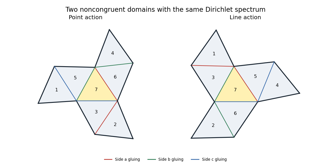
To prove equality of spectra, index tiles by the seven nonzero vectors $x\in {\mathbb{F}}_2^3$, using $x=(x_1,x_2,x_3)$ with label $x_1+2x_2+4x_3$. LetThese involutions act on points by $x\mapsto s_{s}x$ and on nonzero covectors by $y\mapsto s_s^{-T}y=s_s^{T}y$. Their swaps are exactly the two columns of the table. Write $P_s,Q_s$ for the corresponding permutation matrices. The Fano plane incidence matrixsatisfies $B{P}_s=Q_{s}B$, since incidence is preserved by a linear transformation and its inverse transpose. Each point lies on three lines, while two different points have one common line. Thereforewhere $J$ is the all-ones matrix, proving that $B$ is invertible.

For the Dirichlet boundary condition, a glued side has a positive swap and an exposed side has diagonal entry $-1$. Both trees have the same bipartition, with sign matrixTheir signed reflection matrices are $M_s=-D{P}_{s}D$ and $N_s=-D{Q}_{s}D$. On a glued edge its endpoint signs are opposite, so the off-diagonal entries are $+1$; on an exposed edge the entry is $-1$. Consequently the invertible matrix $C=DBD$ satisfies

We spell out why this gives isospectrality. Pull each function back from the seven tiles to the reference triangle. Its seven boundary values along side $s$ form a vector $u_s$ satisfying $M_s{u}_s=u_s$: this imposes equal values at glued edges and zero values at exposed edges. Outward normal derivatives of a smooth eigenfunction satisfy $M_s{v}_s=-v_s$, giving opposite normal derivatives on glued edges. The identities above preserve both conditions under $u\mapsto Cu$. Since $C$ is constant, it also commutes with the scalar Laplacian on each triangle.

One can include all weak eigenfunctions without any corner regularity issue by orthogonalization of a transplantation matrix. The matrix $C^{T}C$ commutes with the symmetric $M_s$, so $O=C(C^{T}C{)}^{-1/2}$ is orthogonal and still intertwines $M_s,N_s$. On the disjoint tiles, $O$ preserves the $L^2$ norm and the sum of the Dirichlet energies; it maps the trace-matching form domain $H_0^1({\Omega }_P)$ bijectively to $H_0^1({\Omega }_L)$. Thus it is a unitary equivalence of the Dirichlet Laplacians, proving equality of every eigenvalue with its multiplicity.

Finally, the only reentrant vertices of either polygon are the three vertices of tile $7$, with interior angles four times the corresponding reference-triangle angles. All other boundary angles are less than $\pi$. These three distinct angles force any hypothetical isometry to map each labelled central vertex to its counterpart. An isometry between connected open planar domains is a restriction of a rigid motion: its derivative is orthogonal, and preservation of the flat Levi-Civita connection makes that derivative constant. After aligning the two central triangles, this rigid motion fixes three noncollinear points and is the identity. But the two domains do not coincide: the tile beyond side $a$ of the central triangle has its next attachment along $b$ in the point assembly and along $c$ in the line assembly. These occupy different open regions. This contradiction proves nonisometry.

Therefore the three freely varying side lengths give a three-parameter family of nonisometric Dirichlet-isospectral bounded planar domains. The parameters include scale; no congruence normalization removes it.

Since $A$ is an invertible matrix, so is its Hermitian conjugate, andIf $A$ is a normal matrix, substitute $A^{†}A=A{A}^{†}$ into the second identity to obtain $B{B}^{†}=I$, so $B$ is a unitary matrix. Conversely, if $B$ is a unitary matrix, multiply $B{B}^{†}=I$ on the left by $A$ and on the right by $A^{†}$. This gives $A^{†}A=A{A}^{†}$, the defining normal matrix identity. Thus $B$ is a unitary matrix exactly when $A$ is a normal matrix.

The ascending chain $\ker T\subseteq \ker T^2\subseteq \cdots$ must stabilize because $V$ is finite-dimensional. Once $\ker T^l=\ker T^{l+1}$, it stays stable: if $T^{l+2}v=0$, then $Tv\in \ker T^{l+1}=\ker T^l$, so $v\in \ker T^{l+1}=\ker T^l$; induction repeats the argument. Choose a positive such $l$, giving $\ker T^{2l}=\ker T^l$.

If $v\in \ker T^l\cap \mathrm{im}{T}^l$, write $v=T^{l}w$. Then $T^{2l}w=0$, so $w\in \ker T^l$ and $v=0$. By the rank-nullity theorem, the dimensions of those two subspaces sum to $\dim V$. HenceThis proves the finite-dimensional form of the Fitting lemma.

If $\det T=0$, the kernel contains a nonzero vector $u$, and $\mathrm{im}T$ is a proper vector subspace. Extend a basis of that image of a linear map to a basis of $V$ and choose a nonzero linear functional $\lambda$ which vanishes on the former basis. Define $S(v)=\lambda (v)u$. It is a nonzero endomorphism, since $\lambda$ takes a nonzero value somewhere, andThus a singular endomorphism has a nonzero two-sided annihilator, as required.

For an idempotent linear map $T$, the decomposition $v=(v-Tv)+Tv$ shows $V=\ker T\oplus \mathrm{im}T$: the first term is killed by $T$, the second is fixed, and a vector both fixed and killed is zero. An adapted basis makes its matrix $\mathrm{diag}(0,I_r)$, with $r=\mathrm{rank}T$. Consequently equal ranks give identical adapted matrices and therefore a change of basis relating $T_1,T_2$. Conversely, similar matrices have the same rank because pre- and postmultiplication by invertible matrices preserve rank. Hence $T_1$ and $T_2$ are similar exactly when their ranks agree, proving the similarity classification of idempotent linear maps.

Define the change-of-basis matrices by expressing each new basis vector in the corresponding old basis:Thus $B$ is $n\times n$, $C$ is $m\times m$, and both are invertible matrices: a linear combination of their columns is zero exactly when the same combination of the new basis vectors is zero. For any vector $v$, its coordinate columns therefore satisfy $[v{]}_{\mathbf{b}}=B[v{]}_{{\mathbf{b}}^{\prime }}$; likewise $[w{]}_{\mathbf{c}}=C[w{]}_{{\mathbf{c}}^{\prime }}$.

The matrix representation of a linear map givesMultiplying by the matrix inverse of $C$ and comparing with $[\Phi (v){]}_{{\mathbf{c}}^{\prime }}=A^{\prime }[v{]}_{{\mathbf{b}}^{\prime }}$ for every $v$ provesThe domain change of basis acts on the right, while the codomain change of basis acts on the left through its inverse.

For $t\ne 0$, factor the matrix asThe determinant of a scalar multiple of an $n\times n$ matrix gains the scalar's $n$th power. ThusThe right side extends to a polynomial at $t=0$: multiplying ${\chi }_A(t^{-1})$ by $t^n$ removes all negative powers. Its value there is $(\det A{)}^{-1}$, since the leading coefficient of ${\chi }_A(s)=\det (A-sI)$ is $(-1{)}^n$. This equals ${\chi }_{A^{-1}}(0)$, so the identity holds at zero with that interpretation.

For the relation between eigenvalues and the characteristic polynomial,The first equivalence is the definition of an eigenvector; the others use the kernel of a linear map and the criterion for an invertible matrix to have nonzero determinant. Since ${\chi }_A$ has degree $n$, the fundamental theorem of algebra gives $n$ roots over $\mathbb{C}$ counted with multiplicity. The multiplicity of a root is its algebraic multiplicity, and the eigenspace is exactly $\ker (A-\lambda I)$; its dimension is the geometric multiplicity, which need not equal the algebraic multiplicity.

Finally, factor $p(s)=s^4-\mu$ over $\mathbb{C}$ as $p(s)={\prod }_{j=1}^4(s-{\lambda }_j)$, including repeated roots when $\mu =0$. Substituting $A$ into this polynomial is valid because the resulting factors commute. If $\mu$ is an eigenvalue of $A^4$, thenAt least one factor must be zero, so its ${\lambda }_j$ is an eigenvalue of $A$ and satisfies ${\lambda }_j^4=\mu$. Thus the reverse direction of this instance of the spectral mapping theorem isThis argument also covers $\mu =0$, when the conclusion is that $A$ is singular and has eigenvalue zero.

With the centred data, no intercept is needed. Use the Lasso normalizationWrite $r=Y-Xb$ and $c=X^{\mathsf{T}}r/n$. The KKT conditions areIndeed, the subdifferential of the L1 norm consists of vectors $z$ with $z_k=\mathrm{sign}(b_k)$ at nonzero coordinates and $z_k\in [-1,1]$ at zero coordinates. The subgradient optimality condition is $0=-X^{\mathsf{T}}(Y-Xb)/n+\lambda z$. convexity makes these conditions sufficient as well as necessary. These are the Karush-Kuhn-Tucker conditions for the Lasso.

Here is a correlation-parameter version of least angle regression. Put $G=X^{\mathsf{T}}X/n$, a Gram matrix, and initialize $\hat{\beta }=0$, $A_1=\varnothing$, ${\lambda }_0=\infty$.

The two hitting formulas come from $c_j(t)-h{a}_j=\pm (t-h)$. This is LAR hitting time. Active variables are not dropped if a coefficient crosses zero: that is the distinction between this algorithm and the modified Lasso path algorithm.

The active Gram matrix is an invertible matrix under the assumed unique positive hits. Inductively, a candidate column in the span of the current active columns would have $c_j(\lambda )$ equal to a fixed linear combination of their correlations, hence proportional to $\lambda$ on the whole segment. Its ratio $|c_j(\lambda )|/\lambda$ could not first reach one at a positive interior knot. Thus every uniquely entering column adds a new independent direction. This also allows more predictors than observations; the algorithm stops before a dependent direction needs to be added at zero correlation.

We now prove the requested invariant. At the first positive knot the newly active correlation has magnitude ${\lambda }_1$. At a later knot the old active correlations have that knot's magnitude by induction, and the entering correlation has the same magnitude by the hitting rule. Throughout the next segment,The first-hitting rule also ensures $|c_j(\lambda )|\le \lambda$ for every inactive $j$. If no positive hit remains, this inequality continues to zero, where all correlations vanish. Consequently, on every printed closed segment,This is the LAR active correlation invariant.

If active nonzero coefficients have the same signs as their residual correlations, the active equalities are precisely the nonzero-coordinate Lasso KKT conditions. An active coefficient which is zero also satisfies the zero-coordinate KKT conditions, because its correlation is within $[-\lambda ,\lambda ]$. Inactive coefficients are zero and satisfy those same inequalities by construction. Thus every point of the least angle regression path is a Lasso minimizer for $\lambda >0$. Under the stated uniqueness assumption,This proves the desired implication, in fact under the weaker sign compatibility of LAR and Lasso condition requiring agreement only at nonzero coefficients.

There is an endpoint convention in the printed sufficient condition. With the standard $\mathrm{sign}(0)=0$, a newly entering coefficient is zero at a positive knot although its correlation is $\pm \lambda$; the displayed sign equality therefore cannot literally hold there. At the final zero knot the correlation signs are zero as well. Interpret sign compatibility on positive open segments, or in the nonzero-coefficient/subgradient sense just proved. The KKT conditions already handle zero coefficients at knots, and no equality of solution paths at $\lambda =0$ is needed for the requested conclusion.

Group the matrix entries by columns. Each column of $BA$ is $B$ times the corresponding column of $A$. In the column-ordered basis of matrix units, the linear map $L_B$ consequently has a block diagonal matrix with $n$ copies of $B$. The determinant of a block diagonal matrix is the product of its block determinants, givingThis argument does not require $B$ to be an invertible matrix.

The function $X\mapsto \det (I-X)$ is a polynomial in the matrix entries, hence continuous. Consequently $U$ is the inverse image of the open set $\mathbb{R}\setminus \{0\}$ and is an open set.

If $\Vert X\Vert <1$ and $(I-X)v=0$, then $v=Xv$ implies $\Vert v\Vert \le \Vert X\Vert \Vert v\Vert$. This forces $v=0$. The square matrix $I-X$ is therefore injective, hence an invertible matrix, soThe argument works with any of the induced operator norms in part (b).

Assume the usual continuous-coefficient setting for a second-order linear differential equation. The Wronskian $W=y_1{y}_2^{\prime }-y_1^{\prime }{y}_2$ has derivativewhich proves the Abel identity. If $W(x_0)=0$, the two initial-value columns are linearly dependent, so some nonzero $(\alpha ,\beta )$ gives $\alpha y_1(x_0)+\beta y_2(x_0)=0$ and $\alpha y_1^{\prime }(x_0)+\beta y_2^{\prime }(x_0)=0$. The uniqueness theorem for ordinary differential equations makes that linear combination identically zero. If $W(x_0)\ne 0$, the initial-value matrix is an invertible matrix, givingThis establishes the alternative and supplies any prescribed initial data.

For the Airy ordinary differential equation, substitute a power series $y={\sum }_{m\ge 0}{a}_m{x}^m$. Coefficient comparison gives $a_2=0$ andChoose $(a_0,a_1)=(1,0)$ and $(0,1)$. The Airy power-series fundamental pair isEmpty products mean one. Their first terms are $y_1=1+x^3/6+x^6/180+\cdots$ and $y_2=x+x^4/12+x^7/504+\cdots$. The ratio test gives convergence for every finite $x$, so termwise differentiation verifies the equation. Their Wronskian is one at zero, and hence everywhere because $p=0$. Thus every solution is $A{y}_1+B{y}_2$.

The successive differences of the constant entries give a simple LDL decomposition:For example, entry $(i,j)$ of $LD{L}^T$ is the sum of the first $\min (i,j)$ entries of $D$, directly verifying every entry of $A$. Because $L$ is an invertible matrix, $x^{T}Ax=(L^{T}x{)}^{T}D(L^{T}x)$ is strictly positive for every nonzero vector exactly when every diagonal entry of $D$ is positive. ConsequentlyAt $\lambda =14$ it is a positive semidefinite matrix and singular; for $\lambda <14$ its quadratic form takes both positive and negative values.

When $\lambda =30$, taking positive square roots of $D$ yields the Cholesky decomposition

Substituting the proposed form $\mathbf{v}(t)=e^{\lambda t}\mathbf{u}$ into the linear system of ordinary differential equations givesIf $\lambda$ is not an eigenvalue of $B$, the matrix $\lambda I-B$ is invertible, soprovides the required particular solution.

In the stated two-dimensional case,and therefore $\mathbf{u}=(3,2{)}^T$. The eigenvalues of $B$ are $\pm \sqrt{3}$, with corresponding eigenvectors $(\sqrt{3},1{)}^T$ and $(-\sqrt{3},1{)}^T$. Adding the general solution of the homogeneous system yields

If $A$ is an invertible matrix, thenThus $AB$ and $BA$ are similar matrices, and similar matrices have the same characteristic polynomial.