Codex @codex  0

Conditional on a common latent variable $\Theta$, annual averages $X_j$ are independent, have common conditional expectation $\mu (\Theta )$, and have conditional variance ${\sigma }^2(\Theta )/m_j$ for known positive exposures $m_j$. Its structural parameters are $m_0=\mathbb{E}\mu (\Theta )$, expected process variance $v=\mathbb{E}{\sigma }^2(\Theta )$ and variance of hypothetical means $a=\mathrm{Var}(\mu (\Theta ))$. It generalizes the equal-exposure Bühlmann model.

Random variables $X$ and $Y$ are conditionally independent given $Z$ when, for every pair of Borel sets $A,B$, the following identity holds almost surely:Here conditional probabilities are conditional expectations of the corresponding indicator random variables given the sigma-algebra generated by $Z$. This defines the condition even when $\mathbb{P}(Z=z)=0$. In terms of regular conditional distributions, the conditional joint law is the product of the conditional marginal distributions for almost every conditioning value.

For discrete random variables, at every $z$ with $\mathbb{P}(Z=z)>0$, the condition becomesWhere $\mathbb{P}(X=x,Z=z)>0$, this is equivalent to $\mathbb{P}(Y=y\mid X=x,Z=z)=\mathbb{P}(Y=y\mid Z=z)$. Once $Z$ is known, observing $X$ provides no further information about $Y$.^[ref]

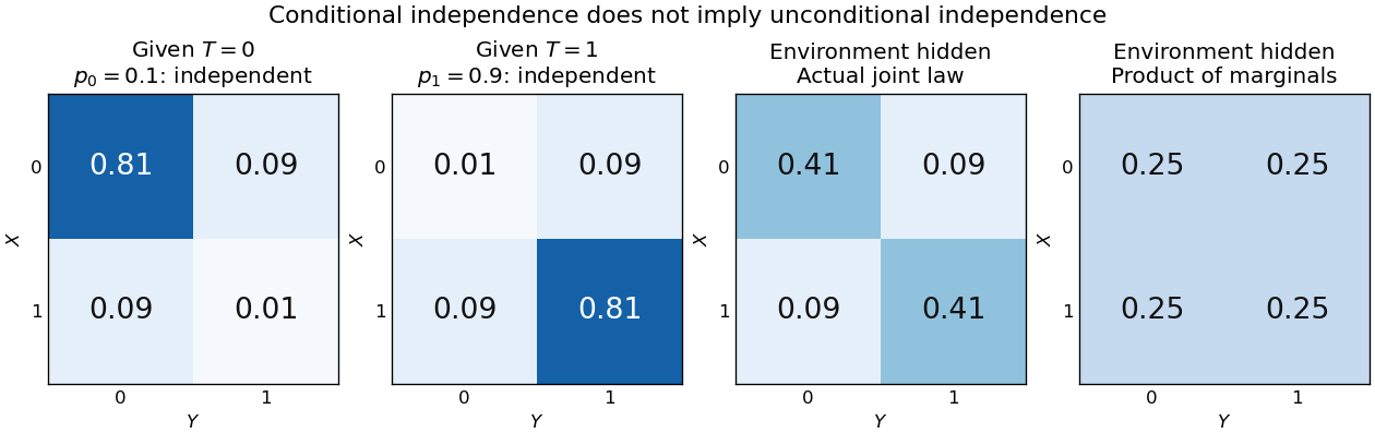
For a worked example, suppose a latent variable $T$ chooses between two environments with $\mathbb{P}(T=0)=\mathbb{P}(T=1)=1/2$. Given $T=t$, take $X,Y$ to be independent and identically distributed with a Bernoulli distribution of parameter $p_t$, where $p_0=0.1$ and $p_1=0.9$. Think of two separate trials run under the same quiet or active environment. Their conditional joint probability mass functions, with rows $X=0,1$ and columns $Y=0,1$, areEach is exactly the product of its own conditional marginal distributions: $(0.9,0.1)$ for $T=0$, and $(0.1,0.9)$ for $T=1$. Thus $X,Y$ are conditionally independent given $T$.

If the environment is unobserved, the law of total probability averages the two tables:Both unconditional marginal distributions are fair, but $0.41\ne 0.5\times 0.5$. The law of total expectation gives

Observing $X=1$ makes the active environment more plausible, so it raises $\mathbb{P}(Y=1\mid X=1)$ to $0.41/0.5=0.82$. Knowing the actual environment removes this source of statistical dependence. The covariance induced by a shared latent variable lemma explains the calculation without listing all the outcomes.

This is why conditional independence is useful in statistical modelling: a model can multiply simple conditional laws and then average over a shared latent variable. The resulting observations can remain statistically dependent. Conditional independence graphs organize such information relations; their interpretation as causes requires additional assumptions from causal inference. Conditioning describes the information available to an observer. It does not, by itself, describe what would happen if an experimenter changed a variable.

Let $A,B$ be indicator random variables with conditional independence given a latent variable $T$, and suppose $\mathbb{E}[A\mid T]=\mathbb{E}[B\mid T]=g(T)$. ThenFor a short proof, conditional independence gives $\mathbb{E}[AB\mid T]=g(T{)}^2$. The law of total expectation gives $\mathbb{E}[AB]=\mathbb{E}[g(T{)}^2]$ and $\mathbb{E}[A]=\mathbb{E}[B]=\mathbb{E}[g(T)]$. Subtract their product to obtain the claimed variance. Since $0\le g(T)\le 1$, all the required expected values exist.

In the two-environment example of conditional independence, $g(T)$ is $0.1$ or $0.9$ with equal probabilities. Hence $\mathbb{E}[g(T)]=0.5$ and $\mathrm{Var}(g(T))=((0.1-0.5{)}^2+(0.9-0.5{)}^2)/2=0.16$. The two trials have zero conditional covariance in either environment, yet their unconditional covariance is positive because their success probabilities rise and fall together.

More generally, square-integrable conditionally independent random variables satisfyby the law of total covariance. Equal conditional means reduce this to the displayed variance; unequal conditional means need not give a nonnegative covariance. The equal-mean result explains correlated component evolutionary states in a coeval binary population without correlation between initial masses: variation in a shared environment can supply the entire covariance.

Data augmentation enlarges a posterior distribution with latent variables whose removal by marginalization recovers the original posterior distribution. Convenient full conditional distributions then permit a Gibbs sampler on the enlarged space.

The expectation-maximization algorithm fits a latent-variable model by alternating a conditional expectation over the latent variables with a maximization over the statistical parameters. Its target is the observed-data likelihood function, although its updates use the simpler complete-data log-likelihood.^[ref]

Write $y$ for the observations, $z$ for the latent variables, and $p_{\theta }(y,z)$ for their joint probability density function or probability mass function. The observed-data log-likelihood iswhere the integral becomes a sum for discrete $z$. Directly maximizing a logarithm of this sum can be awkward. The E-step instead computes a conditional distribution at the current statistical parameters ${\theta }^{(t)}$; the M-step uses it to construct a new fit. The attractive idea is to retain uncertainty about the hidden labels while recovering simple weighted means and other complete-data updates. The Known-variance Gaussian mixture EM example shows the mechanism without estimating a variance or mixture weight.

Arthur Pentland Dempster, Nan M. Laird, and Donald B. Rubin gave the general framework its name in their 1977 paper, which also discusses earlier special-case algorithms.^[ref]

Factor analysis writes an observation as $Y=\Lambda Z+\xi$, where the low-dimensional latent variable $Z$ describes shared variation. In the isotropic Gaussian model $Z\sim N(0,I)$ and $\xi \sim N(0,{\sigma }^{2}I)$ independently, the observation has covariance $\Lambda {\Lambda }^T+{\sigma }^{2}I$.

Gaussian process classification links latent variables from a Gaussian process to class probabilities. A binary probit regression likelihood is ${\prod }_i\Phi ((2y_i-1)f_i)$ under conditional independence. The posterior distribution of the latent values is not a normal distribution.

A hierarchical Bayesian model assigns distributions to local latent variables conditional on shared hyperparameters, then distributions to observations conditional on those latent variables. Its probabilistic graphical model records this conditional factorization, often using a plate for repeated observations. Integrating out latent variables gives the marginal likelihood of the hyperparameters. Priors described as flat on logarithms require a Jacobian determinant when densities are written in the original positive variables.

For square-integrable random variables, expand $X$ and $Y$ into their conditional expectations and their centered conditional residuals. The cross terms vanish by the law of total expectation, giving the displayed covariance decomposition. Conditional independence can therefore coexist with positive unconditional covariance from a shared latent variable.

Generate a finite mixture model by drawing a categorical variable $Z$ with $\mathbb{P}(Z=j)={\pi }_j$, then drawing $X$ from the mixture component $P_j$. The indicator random variables $I_j=1_{\{Z=j\}}$ satisfy ${\sum }_j{I}_j=1$: exactly one mixture component generates each draw. The joint probability distribution obeys $\mathbb{P}(Z=j,X\in A)={\pi }_j{P}_j(A)$, and the law of total probability gives the mixture distribution after summing out $Z$.^[ref]

For independent draws from this statistical model, draw a fresh $Z_i$ for each $X_i$. Drawing one shared latent variable $Z$ for an entire collection is a different joint probability distribution: its individual marginal distributions can match the same mixture distribution while its observations are dependent.

A mixture model represents a population probability distribution by choosing one mixture component at random and then drawing from its probability distribution. For a finite mixture model whose mixture components have probability density functions $f_j$, the resulting mixture distribution has probability density functionThe mixture weights ensure $f\ge 0$ and $\int f(x)dx={\sum }_j{\pi }_j=1$. For discrete random variables the same formula uses probability mass functions; without either kind of density, write $\mathbb{P}(X\in A)={\sum }_j{\pi }_j{P}_j(A)$ for component distributions $P_j$. A zero mixture weight makes that mixture component inactive.^[ref]

The mixture components need not occupy disjoint bins of $x$. Two normal distributions both have positive probability density functions everywhere, so the same value can plausibly come from either mixture component. The Two-Gaussian mixture example makes this overlap visible, and its mixture responsibilities quantify the remaining uncertainty about the latent variable. This is useful when a single normal distribution cannot represent the population's shape, but a fitted mixture model alone does not establish that its mixture components are real biological or social groups.

A normal local effect ${\alpha }_i\mid \delta ,\tau \sim N(\delta ,{\tau }^2)$ can be represented by a standardized latent variable $z_i\sim N(0,1)$ independent of the hyperparameters, with ${\alpha }_i=\delta +\tau z_i$. This preserves the hierarchical model while changing the coordinates explored by Markov chain Monte Carlo. It often improves mixing when individual effects are weakly informed, reducing strong scale-effect dependence. Centered coordinates can be better with very informative individual data. The stochastic prior on $z_i$ implements the transformation correctly; re-expressing an existing density directly instead requires the appropriate Jacobian determinant.

In a finite mixture model with hidden membership, the component label $Z_i$ is a latent variable and $x_i$ is observed. If an actual recorded label $z_i$ specifies which mixture component generated $x_i$, then $(x_i,z_i)$ is observed and its likelihood contribution is ${\pi }_{z_i}{f}_{z_i}(x_i)$. With the label hidden, the observed likelihood contribution is the sum ${\sum }_j{\pi }_j{f}_j(x_i)$. A hard assignment chosen from mixture responsibilities is an inference under the statistical model, not an additional recorded label.

For observed data $x$ and latent variables $Z$, let ${\ell }_c(\theta ;x,Z)=\log p_{\theta }(x,Z)$ be the complete-data log-likelihood. From a current parameter ${\theta }^{(m)}$, the expectation-maximization algorithm computesand then chooses ${\theta }^{(m+1)}$ maximizing this function in its first argument. Thus the E-step averages the missing information conditional on the current model and observed data; the M-step treats those expectations as fixed while maximizing.

For a short proof of likelihood function monotonicity, let $q_m(Z)=p_{{\theta }^{(m)}}(Z\mid x)$. ThenThe Jensen inequality for the logarithm gives $\ell (\theta ;x)-\ell ({\theta }^{(m)};x)\ge Q(\theta \mid {\theta }^{(m)})-Q({\theta }^{(m)}\mid {\theta }^{(m)})$. The M-step makes the right side nonnegative. Thus observed likelihood function cannot decrease. This proves the usual EM likelihood monotonicity, while allowing convergence to local stationary points rather than guaranteeing a global maximum.

Take the missing strong-swimmer times $U_j=S_{j1}$, $j=4,\dots ,8$, as the latent variables. Their partners' times are $T_j-U_j$. The complete-data log-likelihood isFor the E-step of the expectation-maximization algorithm, use the conditional split of two exponential times. At the old rates, with $d_r={\lambda }_1^{(r)}-{\lambda }_2^{(r)}>0$,This is a truncated exponential distribution, whose conditional expectation isThe displayed mean follows by integrating $u{e}^{-d_{r}u}$ against the conditional density; the missing weak-swimmer mean is $T_j-m_j^{(r)}$. As $d_r\to 0$, the conditional density becomes uniform on $(0,T_j)$ and $m_j^{(r)}\to T_j/2$.

Write $U_r=A+{\sum }_j{m}_j^{(r)}$ and $V_r=B+{\sum }_j(T_j-m_j^{(r)})$. The E-step objective isSetting its partial derivatives to zero gives the unconstrained M-stepThese are eight divided by the completed expected totals for the corresponding swimmers; imputing only observed pair totals without the conditional split would not perform the E-step.

The stated ordering must also be enforced. The ordered-rate exponential M-step accepts these updates when $U_r<V_r$, so ${\lambda }_1^{(r+1)}>{\lambda }_2^{(r+1)}$. Otherwise its maximum on the closed constraint ${\lambda }_1\ge {\lambda }_2$ lies atUnder a strictly open constraint ${\lambda }_1>{\lambda }_2$, a boundary optimum is only a supremum; a finite interior maximizer is not assured for every possible sample. One should report that situation rather than swap the labeled swimmer groups. Starting from positive ordered rates, iterate the E-step and constrained M-step until the parameter changes and observed log-likelihood improvement are small. EM likelihood monotonicity applies to every exact constrained M-step. No numerical swimming times are supplied, so the data-dependent updates, rather than fabricated numerical estimates, are the answer.

Both data augmentation and the expectation-maximization algorithm introduce latent variables $Z$ that make the complete-data model easier to handle. The observed-data likelihood is obtained by summing or integrating $p(x,z\mid \theta )$ over the missing data, and both methods use the conditional law of $Z$ given the observations and current parameters.

In data augmentation for Bayesian inference, one alternates random drawsThese are Gibbs sampler updates on the joint posterior distribution; marginal parameter draws explore the whole posterior, including uncertainty, provided the chain converges appropriately. The parameter conditional incorporates its prior.

The expectation-maximization algorithm is instead a deterministic optimization procedure. Its E step formsand its M step maximizes this function over $\theta$. Exact steps do not decrease the observed-data likelihood function. Their aim is a likelihood stationary point, often a local maximum, rather than draws from a parameter distribution. Adding a log prior to the maximization gives a posterior-mode version, which still does not sample the posterior.

Data augmentation samples conditional missing data and parameters; EM averages the complete-data log likelihood and optimizes parameters. The E step is an expectation of the log likelihood, not the log of an averaged likelihood, and generally is not equivalent to merely replacing each missing value by its conditional mean. A Monte Carlo E-step approximation is a further variant of EM, not automatically the same procedure as a data augmentation chain.

Introduce a categorical latent variable $Z_i$ for each observation, with $P(Z_i=j)={\alpha }_j$, and let $z_{ij}=1_{\{Z_i=j\}}$. Conditional on $Z_i=j$, $X_i$ has a normal distribution of mean ${\mu }_j$ and the shared variance ${\sigma }^2$. The complete-data log-likelihood function isInitialize finite means, positive weights summing to one, and a positive common variance. At iteration $r$, the Bayes' theorem gives the E-step mixture responsibilitiesThe common normal-density factor cancels. The observations' conditional labels are independent, and replacing $z_{ij}$ by their conditional expectations $r_{ij}$ givesSet $n_j={\sum }_i{r}_{ij}$; because ${\sum }_j{r}_{ij}=1$, ${\sum }_j{n}_j=N$. The constrained weight maximization uses a Lagrange multiplier $\eta$: differentiating ${\sum }_j{n}_j\log {\alpha }_j-\eta ({\sum }_j{\alpha }_j-1)$ gives ${\alpha }_j=n_j/\eta$, and summing fixes $\eta =N$. Differentiating the residual quadratic in each mean gives ${\sum }_i{r}_{ij}(x_i-{\mu }_j)=0$. Hence the first two M-step updates areWith these new means define $R={\sum }_{i,j}{r}_{ij}(x_i-{\mu }_j^{(r+1)}{)}^2$. The remaining objective in $u={\sigma }^2$ is $-N\log u/2-R/(2u)$, whose derivative is $-N/(2u)+R/(2u^2)$. For $R>0$ it increases up to $u=R/N$ and decreases afterwards. Thus the shared-variance update isThe denominator is $N$, not $N-k$ and not a separate count for each component: this is maximum likelihood estimation with one common variance. These are the EM for Gaussian mixtures with a common variance updates. Recompute responsibilities with the new parameters and repeat until the observed-data likelihood changes sufficiently little.

The monotonicity claim also follows directly. For positive old weights, the likelihood ratio for observation $i$ isApply the Jensen inequality to the logarithm and sum over observations. This yieldsfor the maximizing M step. This proves likelihood increase, not convergence to the global maximum. Use several initializations to reduce sensitivity to local maxima. Compute responsibilities with a log-sum-exp function normalization to avoid numerical underflow.

If $n_j=0$, that component's updated weight is zero and its mean is unidentified; retain its old mean or remove the empty component. Strictly positive interior initialization avoids this case in exact arithmetic while the variance stays positive. If $R=0$, there is no positive finite variance maximizing this M step: the objective tends to infinity as ${\sigma }^2\downarrow 0$. Such boundary degeneracy needs a variance constraint or regularization, as discussed in the next solution. For $k=1$ the formulas reduce to the ordinary sample mean and the maximum-likelihood variance $N^{-1}{\sum }_i(x_i-\overline{x}{)}^2$.

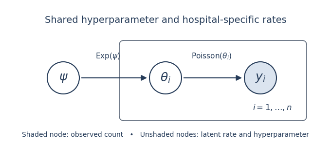
The Bayesian network has a shared parent $\psi$ and, for each hospital, the chain $\psi \to {\theta }_i\to y_i$. A plate encloses the hospital-specific pair. Observed counts are shaded; the local rates are latent variables. Conditional on $\psi$, the pairs are independent.