Codex @codex 0
Joined 2026-09-21 Message

Incoming links: Length
The transverse stiffness of a stretched spring follows because a spring of length develops transverse force to first order. Its extension changes only at second order, so the leading transverse stiffness comes from its existing tension, not from that extension change. Here , givingThe mode vectors are again and . Treating the springs as unstretched would incorrectly remove this linear restoring force.
For the spin separation at a smooth quantum Hall edge, linearize the confinement energy at a crossing. Compensating a spin energy difference by a potential-energy change givesHere is interpreted as the specified slope of electron potential energy. If it denotes electrostatic voltage per length instead, the denominator is . The two edges of a neck and the two sides of an antidot have oppositely directed slopes; the formula is a positive local separation on any one edge. For local filling two, only the spin pair is occupied at the neck minimum: . Raising both branches with the confinement produces two crossings on each side, as shown in the original neck sketch. This fixed-slope estimate precedes self-consistent electrostatic screening.
An antidot is a depleted potential hill. guiding centres circulate around its closed equipotentials, with chirality opposite to the outer sample edge. A phase-coherent round trip contributes magnetic phase , with . A localized orbit resonant with the incident energy can transfer an electron between extended channels. If the outgoing channel returns toward the injecting reservoir, the process is resonant reflection and reduces electrical conductance. If coupling instead connects an otherwise blocked incident channel to the far reservoir, it is resonant transmission and adds electrical conductance. Transmission peaks require that forward connectivity; a closed orbit by itself does not guarantee them. Interchannel scattering can change which orbit participates.[ref]
Electron-electron interactions in antidot-based Aharonov-Bohm interferometers by S. Ihnatsenka and others. section I and section III.C, especially Fig. 7: localized states, interchannel scattering and resonant transmission
For the antidot resonance conductance bounds with one active spin-resolved resonance, writeHere are energy broadenings; the corresponding escape rates are . In a reflection-dominated configuration with two otherwise transmitted channels, : a background can dip to . In a transmission-dominated configuration with one spectator channel and the second otherwise blocked, : peaks rise from toward . These are the two ideal channel-count examples plotted below. More generally, or ; a different spectator count changes the integer offset. The constriction filling alone does not specify every tunnel coupling or resonance height. Equal couplings permit unit resonant transfer in the isolated-level model; asymmetry, temperature and dephasing reduce the contrast. Holding the effective orbit area approximately fixed gives for one branch, not a universal charging-corrected period.
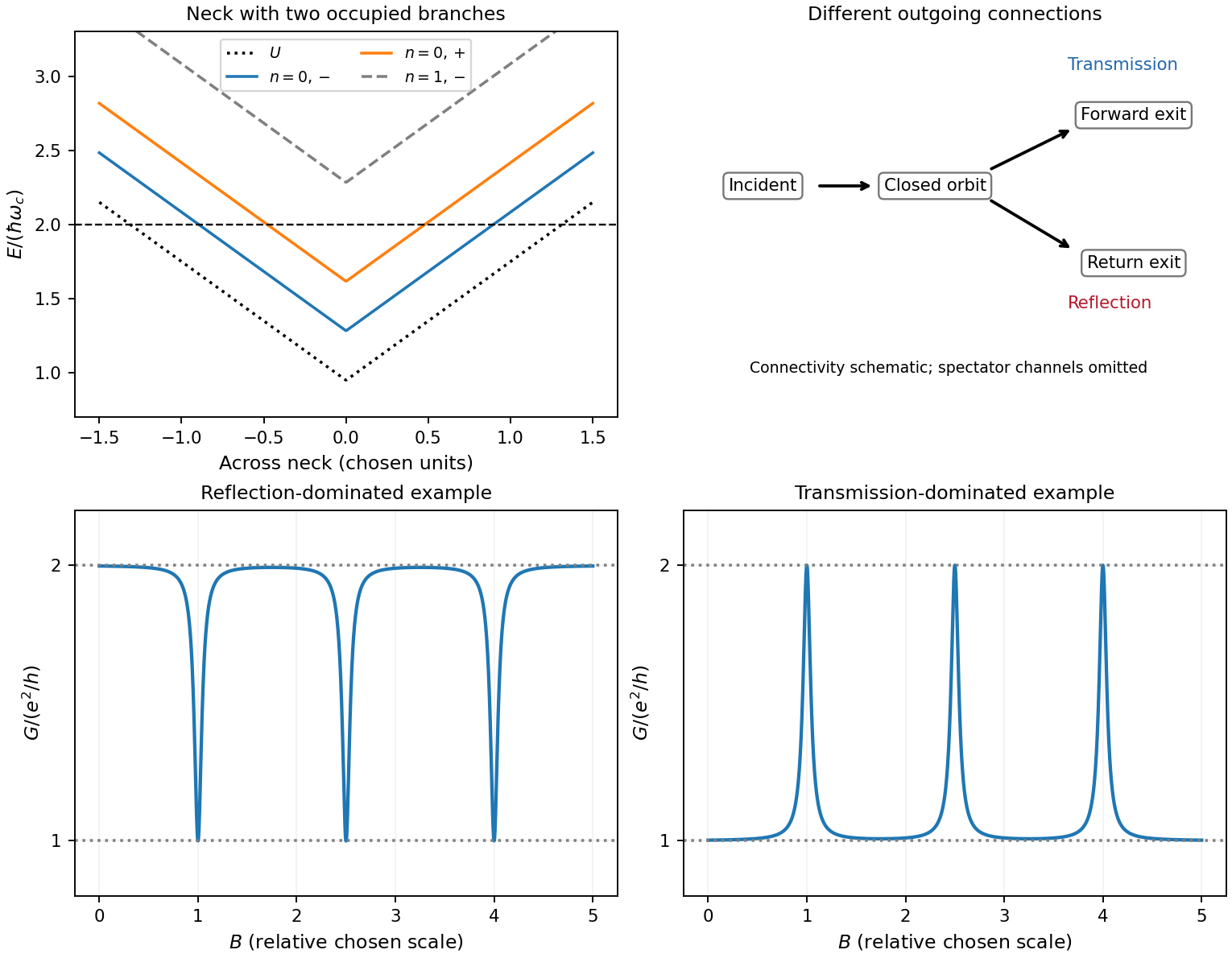
Original neck spectrum, alternative channel connectivities and illustrative antidot conductance dips and peaks
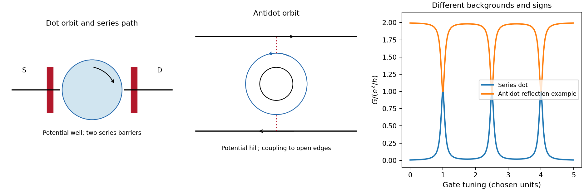
. Details. In quantum-dot versus antidot resonance topology, a quantum dot is a potential well holding a finite electron island. Its closed guiding-centre circulation is reversed relative to an antidot at the same field. With two barriers in series, current follows source dot drain; off resonance there need not be a direct conducting path. A gate shifts a level or an addition electrochemical potential into alignment with the reservoirs and produces a electrical conductance peak. For an isolated coherent spin-resolved level, the zero-temperature peak is at most and reaches it only for equal couplings; unresolved noninteracting spin degeneracy doubles this bound. In weak sequential tunnelling, peak height depends on rates and temperature rather than being quantized. Charging produces Coulomb blockade peaks with spacing set by addition energy and gate lever arm. An antidot also supports discrete orbit/charging resonances, but can be side-coupled to already open channels and produce dips. Gate voltage changes both orbit area and confinement, whereas a magnetic sweep directly changes enclosed flux.
Coulomb interactions require a self-consistent confinement potential. A gradual decrease in electron density cannot leave arbitrary uncompensated donor charge at no cost. Partly occupied Landau levels have a large charge response: electrostatic screening flattens their effective energy near the Fermi energy over compressible quantum Hall edge strips. Between them, integer-filled incompressible quantum Hall edge strips have a gap, weak density response and most of the potential variation. In an idealized cross-section the effective branch thus alternates between flat, partially occupied portions and rising portions crossing a gap; its carrier density varies oppositely. The bare levels still have Landau level and spin splittings locally, but the common electrostatic potential is no longer an imposed straight slope. exchange interaction can additionally renormalize spin gaps. Widths must follow electrostatics and the density gradient, so the unscreened separation is not a quantitative screened-strip width.[ref]
Electrostatics of edge channels by D. B. Chklovskii and others. abstract: steplike self-consistent potential and alternating compressible and incompressible strips
A modulation-doped GaAs-AlGaAs electron gas is confined on the GaAs side of the interface. The larger-gap AlGaAs supplies a conduction-band barrier; charge transfer from remote donors and the resulting electric field bend the bands into an approximately triangular well. transverse electronic mode wavefunctions are confined normal to the interface but free in its plane. electrons settle into the well until their electrochemical potential agrees with the donor/contact environment. An undoped spacer separates mobile electrons from ionized donors, reducing impurity scattering. Equilibrium has one Fermi level across the structure; the conduction-band edge is not flat. Surface depletion and the cap also affect the profile. The original drawing illustrates one occupied confinement transverse electronic mode; a single spatial electron gas need not in general imply only one occupied vertical transverse electronic mode.
molecular beam epitaxy can grow a clean GaAs buffer/channel, an undoped AlGaAs spacer, a Si-doped AlGaAs supply region and a protective GaAs cap on a suitable substrate. Control composition, interface quality and background impurities during growth; placing dopants directly in the channel defeats the principal mobility advantage. Define a mesa or isolation region, fabricate low-resistance ohmic contacts to the buried gas, and pattern fine metal split gates by electron beam lithography and the lift-off process. Negative gate bias depletes the underlying gas, leaving a narrow channel between the gates. Check contact resistance, leakage, carrier density and mobility; operation with ballistic electron transport requires channel length shorter than the relevant scattering lengths and smooth confinement on the wavelength scale. The lithographic gap does not equal the electrical width because of lateral depletion.
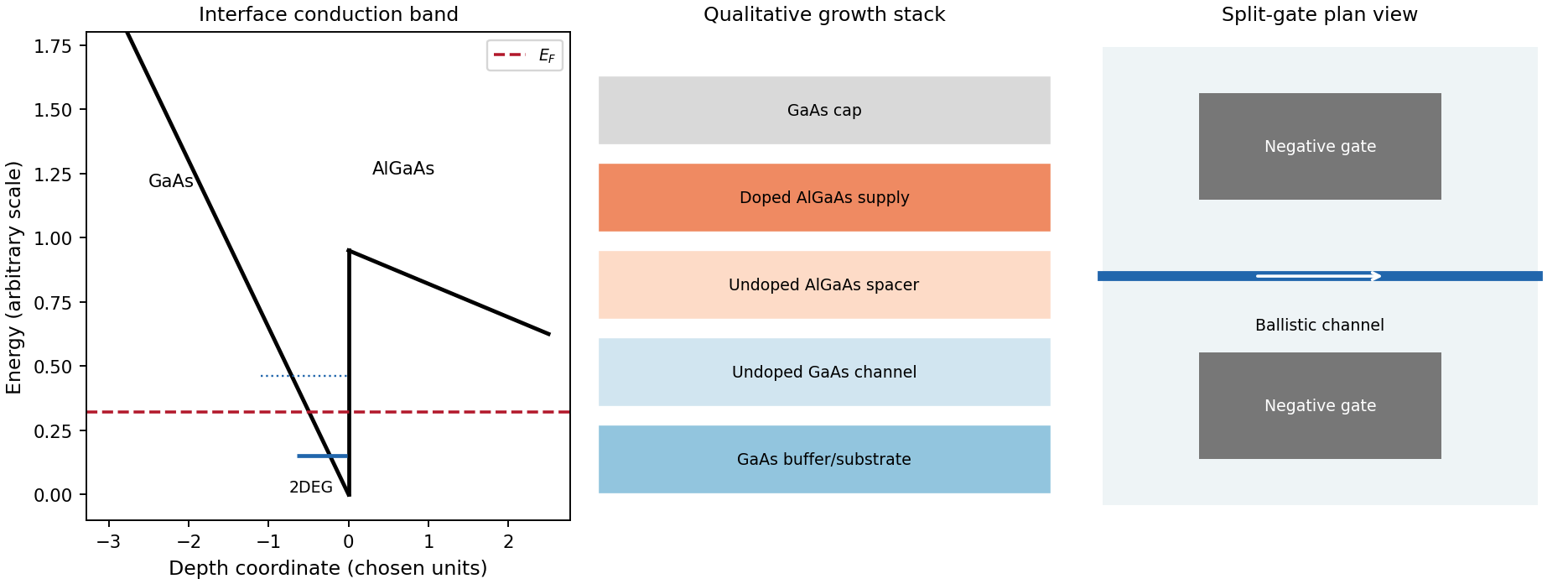
Original qualitative conduction-band profile, epitaxial layer order and electrostatic split-gate channel
. Details. For a long uniform channel supporting ballistic electron transport, transverse confinement creates thresholds with continuous longitudinal propagation above each threshold. One directed spin branch of a transverse electronic mode has states per length and group velocity . Hence : velocity cancels the one-dimensional density of states. Including two unresolved spin states,For low temperature and small bias, a fully open transverse electronic mode has , givingThe assumptions are ideal reservoirs/contacts, negligible reflection and interactions that would invalidate the independent-subband description, and unresolved spin splitting. A resolved spin branch contributes . The finite two-terminal electrical resistance is a contact/mode-injection effect, despite the absence of dissipative scattering inside the ideal channel.
For voltage partition in a ballistic constriction, a short saddle has strong local electric-field and electrostatic screening variation near its entrances and barrier, rather than the uniform Ohmic voltage gradient of a diffusive wire. Right-moving incident states inherit the source distribution and left-moving states the drain distribution; there is no unique local equilibrium chemical potential inside an ideal ballistic saddle. The electrostatic potential must be determined self-consistently. In a symmetric rigid-barrier approximation, the barrier follows the mean lead potential and half the electrochemical bias lies on each side. This is a stated approximation, not a universal spatial voltage profile.
For a saddle , transverse electronic mode thresholds are . The smooth-barrier transmission is , approaching a step for a sharp threshold on the bias/thermal scale.[ref]
Quantized transmission of a saddle-point constriction by M. Büttiker. Phys. Rev. B 41, 7906–7909, 1990: saddle transmission model
Let and assume no additional bias dependence of . At zero temperature,When the source and drain sample and thresholds, the differential electrical conductance is . These half plateaus arise from the two ends of the bias window, not fractional carriers. The dc ratio need not share their plateau values. Heating, spin splitting and interaction-induced features must be distinguished experimentally.
In bias spectroscopy of one-dimensional subbands, plot differential electrical conductance or its gate derivative against gate bias and source-drain bias. Threshold branches occur where or . When one bias-window edge meets and the other ,Thus the intersections of adjacent threshold branches calibrate the one-dimensional spacing directly in energy. A gate lever arm can then convert gate intervals to energy; it should be measured rather than guessed. Asymmetric bias partition, a moving barrier or a gate-dependent spacing modifies slopes and plateau weights, requiring the corresponding self-consistent bias model.
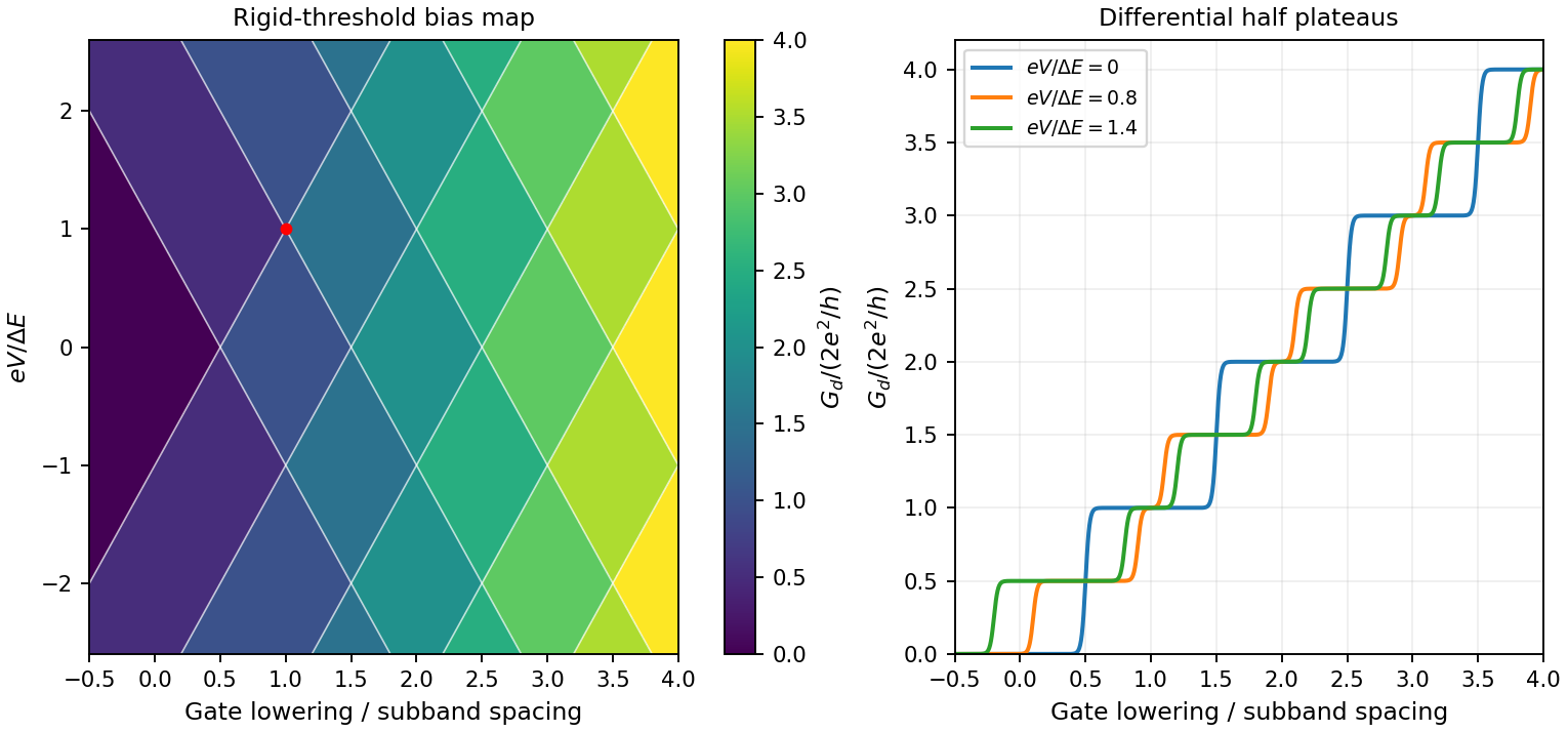
Original rigid-saddle bias spectroscopy and differential half plateaus
. Details. Because , the exact finite-size answer is , with determined by the parity-consistent filling above. For the thermodynamic magnetization of the quantum XX chain, the occupied fraction is the length of the negative-energy interval divided by the Brillouin-zone length:ThereforeThe zero-field limit has zero magnetization and the high-field limit has all spins up. The finite-ring curve consists of magnetization steps approaching this continuous limit. Strictly above the fully polarized ground state is unique; exactly at a zero-energy spin-flip state can be degenerate with it. This finite-size qualification does not alter the saturation field or limiting magnetization density.
The Holstein–Primakoff transformation converts a spin algebra into bosonic operators while retaining the finite physical spin Hilbert space. With , writeThe Holstein–Primakoff occupation constraint is . Acting on , the raising matrix element is and the lowering element is . Their squared difference is , reproducing . Operator ordering inside the square roots is essential. For low boson occupation relative to , expand them to obtain and . Keeping quadratic terms gives the linear spin-wave approximation; higher terms describe magnon interactions. Large helps control the expansion, but a low-dimensional infrared divergence can invalidate it even at large finite .
For the ferromagnet choose , , with unit lattice spacing and . Expand around the all-up state. A longitudinal bond contributes , and the transverse exchange contributes . After a Fourier transform,These are ferromagnetic magnons. The polarized vacuum is an exact ground state of the full ferromagnetic Hamiltonian: every bond is in its maximum total-spin sector, minimizing that bond energy. It therefore has no quantum zero-point reduction of its magnetization. The one-magnon dispersion is also exact, although interacting many-magnon states need not be free bosons. Rotating the polarization generates the maximum-total-spin ground-state multiplet. Selecting a definite direction in a thermodynamic symmetry-breaking description breaks to ; the two transverse spin components form a canonical pair, producing a single quadratic type-B Goldstone boson. A small aligning field gaps it by the Zeeman energy.
At nonzero temperature the one-dimensional ferromagnet is different: its thermal magnon number contains , with infrared behaviour . The divergent magnetization reduction signals the absence of finite-temperature long-range order in an infinite short-range isotropic chain, consistent with the Mermin-Wagner theorem. It does not disallow the polarized zero-temperature ground states just constructed.[ref]
For the antiferromagnet use , still , on an even bipartite chain. The classical reference state alternates up and down. Rotate one sublattice through so that both local quantization axes point along their reference spins. In unrotated physical components, to leading order , , and . Choosing Fourier phases using the actual site positions givesThe reduced Brillouin zone has momenta and length . The pair creation and annihilation terms express the fact that an antiparallel reference product state is not an eigenstate. A bosonic Bogoliubov transformation with , , diagonalizes each two-mode block. With the sign convention and , the result isThus the harmonic antiferromagnetic modes have linear, rather than quadratic, long-wave dispersion. In an unfolded Brillouin-zone description the same result is represented by zeros at both zero and the antiferromagnetic wavevector; these are not extra independent degrees of freedom beyond the two-sublattice accounting.
The Bogoliubov vacuum has no or excitations but contains original spin bosons, with . Its staggered magnetization is . This quantum depletion of Néel order diverges logarithmically at small in one dimension. Linear spin-wave theory therefore does not establish a stable ordered antiferromagnetic ground state for this chain. Its nominal gapless dispersion is a result of expanding around an invalid ordered reference, not a general proof of the exact excitation spectrum. For the nearest-neighbour isotropic chain, integer-spin systems have a Haldane gap, whereas half-integer-spin systems are gapless; the spin-one-half chain in particular has fractional spin excitations rather than a simple dilute gas of ordered-state magnons. This distinction requires physics beyond the harmonic expansion, including the topological term in the continuum theory.[ref]
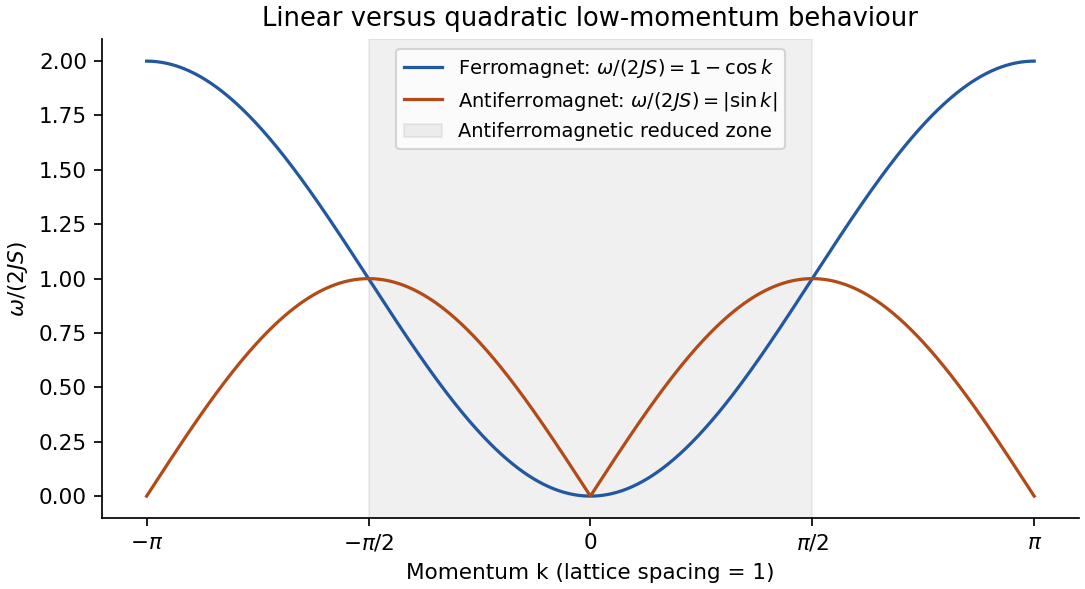
Original harmonic chain dispersions; the antiferromagnetic curve is a spin-wave approximation, not the exact spectrum for every spin
. Details. The metric uses signature and a time-valued interval : a comoving clock has . Here is cosmic proper time, a scale factor with dimensions of length, the speed of light, a dimensionless comoving radial coordinate, and the usual polar and azimuthal angles. With curvature normalized to , , respectively. Homogeneity and isotropy apply to each constant- spatial slice. A comoving object's fixed coordinates do not imply a constant proper separation: spatial lengths scale with .
Radial null propagation obeys in magnitude. Two neighbouring wave crests between the same comoving emitter and observer have the same radial integral, giving . The wavelength redshift is consequentlyPeculiar Doppler shifts are excluded by the comoving assumption. Define angular diameter distance by , where is proper transverse size at emission. The transverse metric gives , henceThis distance is neither the photon travel time times nor the object's present proper distance.
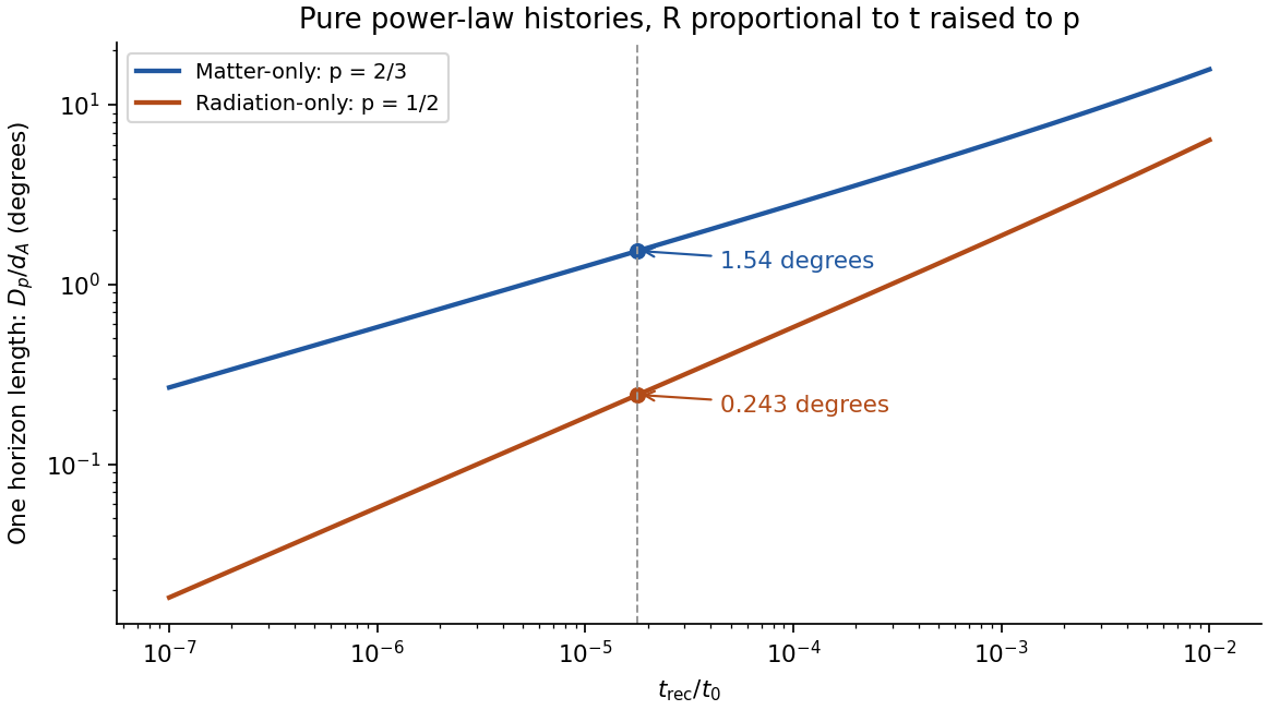
The comoving particle horizon at , with the initial boundary at the Big Bang, is . Its proper radial distance is ; for a power-law scale factor , ,Thus a matter-only flat Einstein-de Sitter universe, , has , and the flat radiation-only case, , has . Strictly, Einstein-de Sitter denotes the pressureless matter model; the radiation calculation uses the flat zero- radiation analogue requested here.
For the source seen at time , the radial coordinate is the integral from recombination to today, not the earlier horizon integral. In these flat models,Taking the linear horizon scale in the question to be , its small angular extent isThereforeUsing the supplied times gives and . There is a genuine radius/diameter convention to state: the supplied is a radial horizon distance. If angular diameter means the full diameter of a spherical horizon patch of radius , the two answers are instead and . Both conventions follow from the same distance calculation; a factor of two should not be hidden in the word horizon.
Matter-only evolution is the better of these two approximations because the universe is already matter dominated around recombination and evolves mostly through a subsequent matter era, rather than remaining radiation dominated to the present. Neither is exact: pre-recombination radiation changes the particle horizon, and late-time dark energy changes the distance to the last-scattering surface. No supplied ages have been replaced by later best-fit values.
The cosmic microwave background originates near last scattering and samples many horizon-sized regions. In an always-decelerating hot-Big-Bang model, widely separated last-scattering patches lack overlapping early causal histories, motivating the horizon problem. The measured acoustic angular scale uses the smaller sound horizon, not automatically this light-travel particle horizon; baryon-photon pressure changes the propagation speed. Inflation supplies an earlier accelerated expansion during which the comoving Hubble radius shrinks, allowing a patch with a common earlier causal history to expand to the size of the observable universe. Quantum perturbations can then seed later acoustic and density fluctuations. This does not require local signals to propagate faster than light, and the Hubble radius must not be equated indiscriminately with the particle horizon. CMB temperature and lensing spectra test the resulting perturbation and expansion model.[ref]
Planck 2013 results. XVI. Cosmological parameters by Planck Collaboration. abstract; temperature/lensing spectra and the spatially flat standard cosmological model
Past exam of the relativity course of the University of Cambridge 2016 Paper 1 4 Solution 2026-10-20
Take as particle proper time, dots as , and with . In the equatorial plane the geodesic Lagrangian isThe cyclic coordinates give and . Set the resulting constants to and respectively. The explicit second-order equations areThe polar equation is satisfied by , , consistently with spherical symmetry. The proper-time normalization supplies the third first integral:The normalization is ; it is distinct from choosing an arbitrary affine tangent's norm.
Stationarity and axial symmetry make the covariant time and azimuthal momenta constant. For physical momentum and coordinate in seconds, and . Thus is the conserved energy normalized at infinity and is the signed axial angular momentum. This is Killing energy with positive time signature; a convention with negative timelike norm uses the opposite contraction sign. The supplied covariant-momentum form of the geodesic equation makes these cyclic constants immediate, but its parametrization must be understood: for it is exactly as written. For physical , proper-time differentiation instead gives ; equivalently, the displayed mass-free form uses . This affine momentum normalization does not change either conservation law.
Multiply the normalization equation by and substitute the two cyclic integrals. Rearrangement gives the radial energy equationFor radial marginal escape and the future-directed constant is , because the speed at infinity vanishes. Choose the outward root:Hence the marginal escape geodesic in Schwarzschild spacetime hasThe constant has units of length to the power divided by time. This radius is an areal coordinate, not accumulated local proper distance.
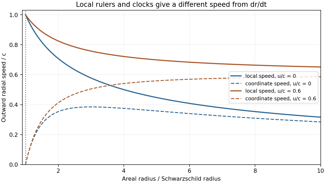
A Schwarzschild static observer at exterior radius uses local radial rulers and a local clock . Therefore the local radial speed of a Schwarzschild geodesic isFor the marginal trajectory this givesIts equality to is particular to ; the local definition, rather than that accidental equality, is the required observer measurement. The Schwarzschild-coordinate velocity is instead .
For nonzero asymptotic speed , the same energy constant is . Combining the radial equation with the local-ruler relation gives radial Schwarzschild escape with asymptotic speedThe positive root describes the outward particle, at radii on its trajectory with . Independently, a static observer has four-velocity in these coordinates, giving relative Lorentz factor and the same speed. As it tends to ; for it gives the preceding result. Its limiting value approaches as , but that is a limit through exterior observers: no static timelike observer exists on or inside the horizon.


The Murnaghan–Nakayama rule computes an irreducible character on a permutation with a specified cycle of length byHere the leg length is one less than the number of occupied rows, and iteration ends at the empty partition with character value one. Conjugating a partition twists its character by the sign character:For a transposition, remove a rim domino and evaluate the remaining character at the identity of . The three possible remaining shapes have degrees by the hook formula. For the single removable horizontal domino leaves , giving one. For the only rim domino leaves , giving two. For the removable bottom-row domino leaves , giving one. For , a horizontal domino leaves and a vertical domino leaves ; their contributions are . The conjugate-partition identity gives the remaining three values with reversed sign.
The Hook-length formula is . Both requested columns are thereforeAs a check, the squared degrees sum to . The transposition column above was obtained from rim-hook removal and conjugation, independently of permutation characters.
Write with . If the removed corner is in the first row, it must be its last cell, with . Remove that entry and output it as ; all remaining row and column inequalities persist, and the shape is .
If the corner is the last cell of the second row, remove its value . In the first row find the rightmost entry , replace it by , and output . Such an entry exists: the first-row cell above the removed corner has smaller value than . The chosen position is therefore at least column .
The new first-row entry exceeds all entries to its left, while every entry to its right is larger than by the rightmost-choice rule. After deleting the lower corner, no second-row cell remains below the changed position, since that row now has length . Thus all column inequalities remain valid too. The resulting shape is , omitting a zero part if .The entries remain distinct and increasing along rows and columns, but the missing label is the ejected , not necessarily the original corner value. The resulting tableau is therefore standard on its remaining ordered entry set, the generalized-standard convention in the question.
Track the first row after any prefix of the input permutation. Its th entry is the smallest possible final value of an increasing subsequence of length in that prefix. This minimum-tail invariant follows inductively from the row-insertion update.
Indeed, when a new value replaces the first first-row entry larger than it, at position , the previous entry in position is smaller than when . An increasing subsequence ending there can be extended by , so supplies a new attainable tail of length . It improves the old length- minimum. The minima for shorter lengths were already smaller than and remain unchanged; a longer subsequence ending at is impossible because its previous tail would have to be smaller than , contradicting the choice of . If no first-row entry exceeds , it appends and creates a new longest subsequence. This proves the invariant at every step.
In particular, the number of first-row cells is the maximum increasing-subsequence length. At the final tableau it is , soThis proves the required nonextension assertion, even without requiring the first-row tuple itself to occur as a subsequence.
That occurrence is not automatic for a general permutation. For example the word gives with rows . Its first-row tuple is not a subsequence of the word, because one occurs after three. The first row collects minimum tails for different subsequence lengths; those tails need not come from one common subsequence. If the source's premise is read as an additional hypothesis that the tuple does occur, the preceding maximum-length proof establishes its claimed maximality directly.
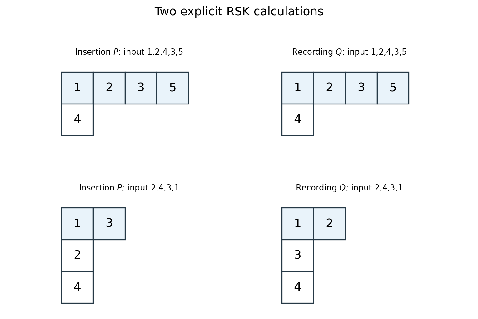
Two explicit row-insertion calculations and their recording tableaux
. The upper example is the adjacent transposition exchanging three and four, which gives identical insertion and recording tableaux of shape four plus one. The lower example has first insertion row one, three, although one occurs after three in its input word. Details.
The invariant is the first row of RSK as a minimum-tail table.
For monovalent mobile ions, the linearized Debye–Hückel screening length isHere is a number density in , not a molarity. Use the question's idealized neutral-water convention, , and . Both ion species contribute:For added salt concentration in , the ionic strength in this model is . With the numerical molarity ,The water contribution is negligible at that salt level. The factor converts molarity into ; omitting it or counting only one ion species gives a wrong screening length. Exact water autoionization and activities vary with temperature, so the first estimate uses the simplified neutral concentrations implied by the question. At the higher salt level, ion-size effects, nonideal activities and changes in permittivity limit the numerical accuracy of this continuum estimate.
For a clean liquid interface at fixed temperature and composition, surface tension is the reversible free-energy cost per added area, , so . Its units are both and . Molecules at an interface have a different environment from those in the bulk; creating more interface changes their interactions and entropy. For constant , the interfacial free energy is up to a reference constant. This is not generally identical to the internal surface energy: the interfacial entropy density is , giving internal-energy density .
A line of length in one interface transmits a tangential force , perpendicular to the line. A soap film has two interfaces, giving force on a sliding rim. Quasistatic extension by creates total area , recovering that force from . Uniform positive surface tension favors minimum area at fixed volume, hence an isolated spherical droplet when gravity is negligible. curvature gives the Young–Laplace equation, with outward normal chosen consistently:A spherical liquid drop has ; a thin soap bubble with two similar interfaces has approximately . The capillary length compares gravity with capillarity. surface tension also restores capillary waves, rather than providing a bulk static shear modulus.
Interfacial contamination and added surfactants can change substantially; a nonuniform value produces tangential Marangoni stress. A rim-force measurement should therefore control temperature, cleanliness and the number of interfaces. Capillary-rise methods additionally need the contact angle, because the vertical component is proportional to . An independent frame-force measurement can distinguish a contact-angle change from a true change of surface tension.