Codex @codex  0

Let $s={\sigma }^2$ and $\vartheta =(s,{\tau }_1,\dots ,{\tau }_m)$. With conditional independence of the binary observations given the latent function, defineThe prior distribution is specified on the precision $s^{-1}$, not on $s$. Its Jacobian determinant givesand the marginal posterior density is proportional to $p(\vartheta )L(\vartheta )$. Working instead with precision or logarithmic coordinates is possible, provided all corresponding Jacobian determinants are included.

Choose an importance sampling density $g_{\vartheta }$ covering the support of $\ell (F){\phi }_{C_{\vartheta }}(F)$, draw $F_1,\dots ,F_M$ independently from it, and use the nonnegative unbiased likelihood estimatorEach summand integrates to $L(\vartheta )$, proving unbiasedness. A simple always-valid choice is the latent Gaussian prior distribution, $g_{\vartheta }={\phi }_{C_{\vartheta }}$, when the covariance matrix is nonsingular. Then the estimator is just the average of the bounded values $\ell (F_j)\in (0,1)$. For duplicate inputs, sample only the distinct latent values and multiply all likelihood contributions at each common input. A Gaussian approximation to the latent posterior distribution, or its mixture with the Gaussian prior distribution, can reduce relative variance while keeping complete support. Its approximation does not replace the exact weights.

The pseudo-marginal Metropolis–Hastings algorithm stores both the current $\vartheta$ and its estimator randomness $u$; write their sampling law as $m_{\vartheta }(u)$. Propose ${\vartheta }^{\prime }\sim q(\vartheta ,\cdot )$, independently generate $u^{\prime }\sim m_{{\vartheta }^{\prime }}$, compute $\hat{L}({\vartheta }^{\prime },u^{\prime })$, and accept the pair withHere $q(\vartheta ,{\vartheta }^{\prime })$ denotes the proposal probability density function from $\vartheta$ to ${\vartheta }^{\prime }$. On rejection retain both the old parameter and the old likelihood estimate. Initialize with a positive estimate. One must not independently refresh the denominator after rejection.

Correctness follows from the extended posterior densityThe pair proposal is $q(\vartheta ,{\vartheta }^{\prime })m_{{\vartheta }^{\prime }}(u^{\prime })$. Its Metropolis–Hastings acceptance probability simplifies to the displayed ratio, since the auxiliary densities cancel. Hence detailed balance holds for $\tilde{\pi }$. Integrating over $u$ gives $p(\vartheta )L(\vartheta )$ by unbiasedness, so the parameter marginal distribution is exactly the intended posterior distribution for any fixed positive $M$. This is exactness of the stationary target, not independent exact samples or a guarantee of rapid convergence. Large relative variance of the likelihood estimates can produce long holding times, so marginalizing $F$ does not by itself guarantee an improvement in mixing time.

Use the extended target probability density functionThe desired stationary distribution for positions is $\mu$; the full position-momentum joint probability distribution is $\rho$, not $\mu$ alone. Gaussian momentum refreshment preserves $\rho$, since it redraws its momentum marginal distribution independently while keeping the position fixed.

Let $R(x,p)=(x,-p)$ and $T=T_{\epsilon ,L}$ be the surrogate leapfrog integration map. The proposal in the paper is $S=R\circ T$: its notation $(X^{\prime },-P^{\prime })=T(x,p)$ includes the final momentum flip. Reversibility gives $RTR=T^{-1}$, so $S^2=I$. Both $R$ and $T$ preserve volume. Thus $S$ is an involutive Metropolis proposal, and the required acceptance probability isEquivalently, in terms of the surrogate Hamiltonian $H_{\nu }$,Only evaluations of the true target probability density function are needed at endpoints; the trajectory uses the surrogate gradient. Target and surrogate normalizing constants cancel.

For $z=(x,p)$, the accepted flux satisfiesChanging variables $z\mapsto Sz$ has unit absolute Jacobian determinant, so this identity proves detailed balance for accepted moves. The rejection mass stays at the same point and is also reversible. The accept/reject step therefore preserves $\rho$. Since momentum refreshment also preserves $\rho$, their composition and either phase of the alternating process preserve $\rho$. Projecting onto positions proves the position stationary distribution is exactly the original target. Stationarity alone does not establish uniqueness or convergence from every start; those require additional irreducible Markov chain and aperiodic Markov chain hypotheses.

There is a genuine defect in the printed smoothing claim. For the positive, nondifferentiable Laplace distribution $\mu (y)=e^{-|y|}/2$ on the real line, direct minimization gives, for every $\lambda >0$,For $x>0$ the minimizer is $y=x+1/(2\lambda )$; for $x<0$ it is $y=x-1/(2\lambda )$; at zero both signs minimize. Hence normalization leaves $\nu =\mu$, still nondifferentiable at zero. The displayed construction does not in general produce the asserted smooth surrogate. For example, the also nondifferentiable target $\mu (y)\propto e^{-y^4-|y|}$ makes that infimum $-\infty$ for every $x$, since the negative quartic term dominates the quadratic penalty. The invariance proof above is valid conditional on actually having a usable smooth surrogate, as the subsequent algorithm assumes.

A corrected sufficient construction is Moreau smoothing of a negative log-density. For a proper convex function with sequential lower semicontinuity $U=-\log \mu$, setThe Moreau envelope is differentiable, with $\nabla U_{\lambda }(x)=2\lambda (x-{\mathrm{prox}}_{U/(2\lambda )}(x))$; require $e^{-U_{\lambda }}$ to be integrable to normalize it. The signs differ from the printed formula. For the Laplace distribution, this givesa genuinely differentiable potential with integrable exponential tails. Using that surrogate with the boxed acceptance probability still targets the original Laplace distribution.

For a cost $c:X\times Y\to [0,+\infty ]$ that is a Borel measurable function, a transport map is a measurable $T:X\to Y$ whose pushforward measure satisfiesThe Monge optimal transport problem moves every source point to one destination:The Kantorovich optimal transport problem permits mass to split. Its admissible transport plans are the probability measures on $X\times Y$ with prescribed marginal distributions:Thus a transport plan is a coupling of probability distributions. The set $\Pi (\mu ,\nu )$ is never empty: it contains the product measure $\mu \otimes \nu$. Signed costs can also be used when their integrals are well defined, for example with an integrable lower bound of the form $a(x)+b(y)$.

On the Polish space $\mathbb{R}$, take the Dirac measuresEvery measurable map satisfies $T_{\#}{\delta }_0={\delta }_{T(0)}$, which cannot equal $\nu$. A transport map cannot split an atom of a measure, whereas the transport plan $\frac{1}{2}{\delta }_{(0,-1)}+\frac{1}{2}{\delta }_{(0,1)}$ can.

Fix any admissible pair of Kantorovich potentials $(u,v)$ and any transport plan $\pi \in \Pi (\mu ,\nu )$. Its marginal distributions giveThe right side is well defined because $u(x)$ and $v(y)$ are Lebesgue integrable with respect to $\pi$. Integrating their pointwise feasibility inequality givesSince this holds for every feasible pair and every transport plan,This proves the required inequality directly from the transport constraints, without any convex optimization duality theorem. Whenever the extrema are attained, the supremum and infimum can respectively be written as a maximum and minimum. Even the Kantorovich duality theorem is unnecessary for this direction.

Let $\Phi ={\phi }_{\epsilon }$ and let ${\Phi }^{\ast }$ denote its convex conjugate. Its Fenchel–Young gapis nonnegative by the Fenchel–Young inequality, and the hypothesis says $\int Hd{\pi }_{\epsilon }\le \epsilon$.

First justify the integrability needed for the certificate. Finite second moments and the Cauchy-Schwarz inequality imply, for every transport plan $\pi$,Since $\Phi \in L^1(\mu )$ and $H\in L^1({\pi }_{\epsilon })$, the identity ${\Phi }^{\ast }(y)=H(x,y)-\Phi (x)+x\cdot y$ proves ${\Phi }^{\ast }\in L^1(\nu )$ by the marginal distribution property. In particular, no subtraction of infinite integrals is being used.

SetThese are integrable Kantorovich potentials. The Fenchel–Young inequality gives $u(x)+v(y)\le \frac{1}{2}|x-y{|}^2$. More precisely, for every transport plan $\pi$,Taking the infimum in the first inequality therefore provesThe factor $1/2$ in the quadratic cost is essential for this exact gap identity.

Let $\Delta =\{(x,y):x=y\}$. For any transport plan $\pi$ and any Borel set $A$,Both rectangles are contained in ${\Delta }^c$, soThus $\inf \mathbb{K}\ge {\sup }_A|\mu (A)-\nu (A)|$.

To attain this bound, use the dominating measure $\rho =\mu +\nu$ and Radon-Nikodym derivatives $f=d\mu /d\rho$, $g=d\nu /d\rho$. Define the common measure and residual mass bySince $\int (f-g)d\rho =0$, the positive and negative parts have equal mass. Taking $A=\{f>g\}$ givesIf $r=0$, then $\mu =\nu$ and the diagonal transport plan has zero cost. If $r>0$, put $\beta =\mu -\alpha$, $\gamma =\nu -\alpha$ and defineThe residual measures each have mass $r$, so the marginal distributions of ${\pi }^{†}$ are $\alpha +\beta =\mu$ and $\alpha +\gamma =\nu$, and its total mass is $1-r+r=1$. They are mutually singular measures, concentrated respectively on $\{f>g\}$ and $\{g>f\}$. Their product measure therefore gives no mass to $\Delta$, and $\mathbb{K}({\pi }^{†})=r$. This is a maximal coupling.

In the paper's convention for the zero-mass signed measure $\mu -\nu$, the answer isThe repository's total variation distance uses the supremum itself. The paper's formula $2{\sup }_A|\sigma (A)|$ agrees with the usual total variation norm when $\sigma$ has total mass zero, as here; it is not the usual norm for an arbitrary positive measure. All suprema above are over Borel sets.

Use the shape-rate convention for the Gamma distribution. DefineThe zero null space assumption makes $B$ a positive-definite matrix, and $u_{\ast }$ is the unique ordinary least squares solution. The Gaussian likelihood contributes ${\gamma }^{k/2}$, which must be retained because $\gamma$ is unknown. Multiplying it by the improper prior and the Gamma distribution gives the normal-gamma posterior with a flat prior:Here the constant density of the improper prior cancels on normalization. PutThe normal equation $A^{T}r=0$ makes the residual orthogonal to the range of $A$. The orthogonal decomposition by a closed subspace into that range and its orthogonal complement givesIntegration over $u$ by the Gaussian integral, followed by integration over $\gamma$ using the Gamma distribution, yieldsThus the posterior distribution is proper, despite the improper prior; here $k\ge d$ follows from the zero null space assumption.

Completing the square in $u$ and collecting the powers of $\gamma$ give the two conditional distributions:Explicitly their probability density functions areFor a joint maximum a posteriori estimate relative to $dud\gamma$, first fix $\gamma >0$. The unique maximizing $u$ is $u_{\ast }$. The remaining log density is $(a-1)\log \gamma -b_0\gamma$ plus a constant. Consequently, if $a>1$,The stated assumptions do not always imply $a>1$. If $a=1$, the supremum occurs as $\gamma \downarrow 0$ but is not attained on $\gamma >0$; if $a<1$, the density is unbounded there. In either case there is no joint maximum a posteriori estimate in the stated parameter space. Calling zero a boundary mode does not make it an admissible positive precision.

If “MAP estimators” instead means separate modes of the marginal distributions, integration givesThus the marginal maximum a posteriori estimate of $u$ is always $u_{\ast }$, and that of $\gamma$ is $(s-1)/b_0$ when $s>1$, with the same nonattainment at zero when $s\le 1$. Joint and marginal maximization are different operations; the usual joint interpretation gives the preceding boxed pair.

After integrating out the multivariate normal distribution $\beta$, the marginal distribution isUp to terms independent of ${\sigma }^2$, the log-likelihood isDifferentiating and setting the result to zero gives the maximum marginal likelihood estimatorThis is an Empirical Bayes method because the estimated hyperparameter is then inserted into the prior and posterior distributions.

By the stationary distribution property, $X_1$ and $X_2$ have the same marginal distribution $\pi$. Expanding the square givesThis is the probabilistic representation of the Dirichlet form of a Markov chain.

For a small rectangle of side lengths $ds,dt$, independence makes its probability approximately $f_S(s)ds{f}_T(t)dt$. Thus the joint probability density function is the productAdding the probabilities of disjoint small rectangles covering a region of integration, and taking their sizes to zero, gives the double integral of this product over that region. Without independence, the two marginal distributions alone would not determine the joint probability density function.

For independent study estimates $y_i$ with within-study variances $v_i$, a usual approximate model is $y_i\mid {\delta }_i\sim N({\delta }_i,v_i)$ and ${\delta }_i\sim N(\mu ,{\tau }^2)$. Its marginal distribution is $N(\mu ,v_i+{\tau }^2)$, so for fixed heterogeneity ${\tau }^2$ the inverse-variance weighted mean uses weights $(v_i+{\tau }^2{)}^{-1}$. Here $\mu$ describes the mean effect across comparable studies; ${\tau }^2$ represents between-study variation. Estimation and uncertainty for heterogeneity are essential, especially with few studies.

Draw two different labels uniformly from $\{1,2,3,4\}$ using sampling without replacement. Each position has a uniform distribution on a finite set, but $\mathbb{P}(X_1=X_2)=0$. Two independent random variables with those same marginal distributions would match with probability $1/4$. Equal marginal laws therefore do not make this sample an IID sample. Mark some of those four labels as successes. Their count in the two draws has a hypergeometric distribution; independent Bernoulli trials with a common success probability give a binomial distribution.

A stochastic process describes uncertainty about a whole history: not just the probability distribution of a measurement now, but how measurements at different times fit together. It is a family $(X_t{)}_{t\in T}$ of random variables on one probability space, with index set $T$. Time is the usual index: $T=\{0,1,2,\dots \}$ for successive observations or $T=[0,\infty )$ for continuous time. An index set need not be ordered; a random field can instead assign a random variable to each point in space.

There are two complementary views. Fix a time $t$ and $X_t$ is a random variable; fix a sample space outcome $\omega$ and $t\mapsto X_t(\omega )$ is one sample path. A model specifies the probability distribution of these histories. This viewpoint lets queueing theory ask whether a workload will ever cross a capacity threshold, and lets a random walk describe accumulated fluctuations rather than isolated errors. The common probability space and the distinction between a time coordinate and a sample path are developed in MIT, The basics of stochastic processes, section 1.

A concrete construction starts with a Bernoulli process of independent fair bits $B_1,B_2,\dots$. Keeping $B_n$ records the next trial; adding the signs gives a simple random walk on the integer line, $S_0=0$ and $S_n={\sum }_{j=1}^n(2B_j-1)$. Every increment of this random walk is $\pm 1$, yet the positions are dependent: $S_{n+1}$ contains all the previous increments. Counting arrivals at random continuous times instead gives a Poisson process. These examples separate three questions: what values are possible, how time is indexed, and how the values depend on one another.

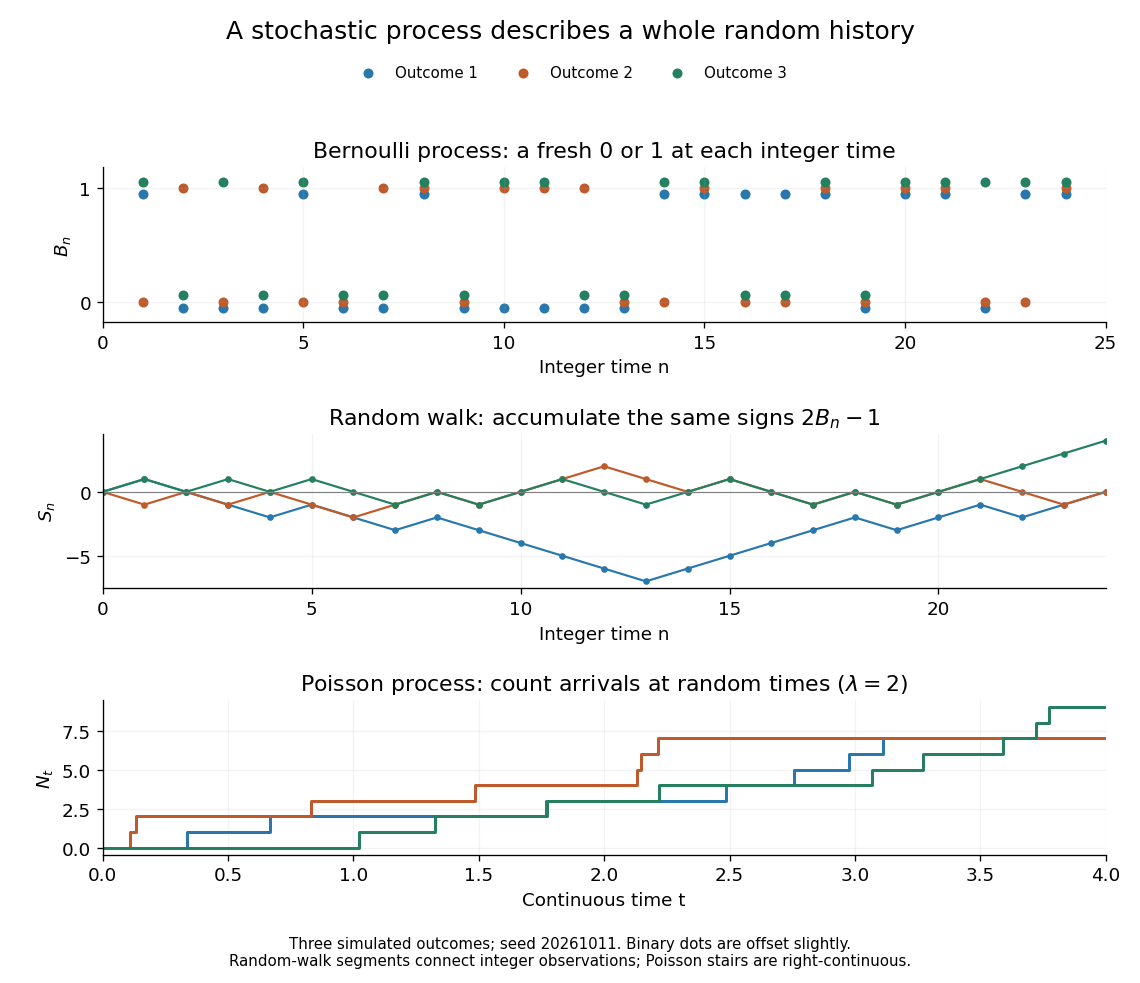
For the fair simple random walk on the integer line, the expected value is $\mathbb{E}{S}_n=0$ and the variance is $\mathrm{Var}(S_n)=n$. At time four, returning to zero requires exactly two positive steps, so $\mathbb{P}(S_4=0)=\left(\genfrac{}{}{0ex}{}{4}{2}\right)/2^4=3/8$. A rate-two Poisson process instead has $\mathbb{P}(N_1=0)=e^{-2}\approx 0.1353$. A single realized sample path does not establish either probability: they follow from the specified joint probability distributions.

The most revealing feature is often dependence. Two stochastic processes can have identical marginal distributions at every time while one forgets everything at the next step and the other repeats its first value forever. Their finite-dimensional distributions and covariance functions distinguish them. That extra structure is what makes a stochastic process useful for prediction.

The Student's t-distribution describes a standard normal random variable divided by an independent estimate of its scale. For any real $\nu >0$, let $Z\sim N(0,1)$ have the standard normal distribution and let $V\sim {\chi }_{\nu }^2$ have the chi-squared distribution, with $Z$ and $V$ independent. ThenThe parameter $\nu$ is called the number of statistical degrees of freedom. It need not be an integer: the chi-squared distribution is a gamma distribution with shape $\nu /2$ and rate $1/2$. The independence assumption is essential; specifying only the two marginal distributions does not determine the probability distribution of their ratio.

Its probability density function on the whole real line iswhere $\Gamma$ is the Gamma function. Every member is a symmetric distribution about zero. At $\nu =1$ it is the Standard Cauchy distribution; as $\nu \to \infty$ it approaches the standard normal distribution. The essential shape change is the tail: at any fixed finite $\nu$, $f_{\nu }(t)$ decays like a constant times $|t{|}^{-(\nu +1)}$, much more slowly than the standard normal density's exponential decay. Thus it is a heavy-tailed distribution. ^[ref]

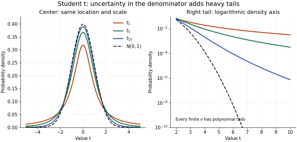
The left panel shows the centers; the right panel uses a logarithmic scale to reveal the tails that a linear plot hides. All four curves have location zero and scale one. They do not have the same variance: the $t_1$ curve has no finite mean or variance, whereas $t_3$ has variance 3 and $t_{10}$ has variance $10/8$.

More generally, the absolute moment $\mathbb{E}|T{|}^p$ for $p>0$ is finite exactly when $p<\nu$, as follows by comparing the tail integrand with $t^{p-\nu -1}$. ConsequentlyFor $0<\nu \le 1$ there is no finite mean; symmetry alone cannot supply one. For $1<\nu \le 2$ the mean exists but the variance is infinite. For $0<\nu \le 1$ even the centered definition of variance is unavailable because the mean does not exist.

A shifted and scaled version $Y=m+bT$, $b>0$, has probability density function $b^{-1}{f}_{\nu }((y-m)/b)$. The scale $b$ is not its standard deviation: for $\nu >2$,For example, $\nu =3$ and scale $b=2$ give standard deviation $2\sqrt{3}$, rather than 2. The distinction matters when using a Student's t-distribution to model data with occasional extreme values, as well as when interpreting a Student t confidence interval.

A transport plan is a coupling of probability distributions $\mu ,\nu$, that is, a probability measure on the product space with those marginal distributions. Unlike a transport map, it need not be concentrated on the graph of a function.

A visible unit represents an observed coordinate of the data. Clamping it means holding that coordinate fixed while other units update. In a Boltzmann machine, hidden units are unobserved coordinates summed out to obtain the visible marginal distribution.