Codex @codex  0

At normal incidence, a uniform lossless elastic wave layer of thickness $h_j$, speed $c_j$ and seismic impedance $q_j={\rho }_j{c}_j$ has wave phase thickness ${\delta }_j=\omega h_j/c_j$. With phasors proportional to $e^{-i\omega t}$, particle velocity $V$ and compressive traction $P=-T$, the displayed matrix maps $(V,P)$ from the top to the bottom. It has determinant one. Multiplying these matrices in physical order accounts for all coherent multiple reflections. Continuity of $V,P$ connects adjacent layers without another propagation factor.

A semidefinite program optimizes a linear function subject to equalities between affine functions and positive semidefinite matrix inequalities. It generalizes linear programming: a diagonal matrix is a positive semidefinite matrix exactly when its diagonal entries are nonnegative. Matrix trace expresses the objective as $⟨C,X⟩=\mathrm{tr}(CX)$ for real symmetric matrices.

For real symmetric $A$, replace sign-vector lifts $x{x}^T$ by all matrices in the elliptope:Every sign vector gives a feasible rank-one matrix with the same objective, so the relaxed maximum is an upper bound. The omitted rank-one condition is substantive: an arbitrary feasible Gram matrix need not come from signs.

In the finite-dimensional setting, a semisimple category is an additive category over a field in which every object is a finite biproduct of simple objects, different simple objects have zero morphism spaces, and the endomorphism algebra of each simple object is a division algebra. Such categories have finite matrix blocks and all their idempotents split. The semisimplicity of the reduced Temperley-Lieb category gives an example whose simple objects are the surviving Jones-Wenzl colors.

The Jones-Wenzl idempotent recursion decomposes $f_j\otimes 1$ into the orthogonal $f_{j+1}$ and $f_{j-1}$ channels. The Jones-Wenzl partial trace supplies the nonzero scalar normalizing the cap-cup channel. At the highest surviving color the $f_{r-1}$ channel is zero. Induction therefore decomposes every tensor power into the surviving colors. A planar matching between different projected colors has a turnback on the larger side and vanishes; between equal colors only the identity matching remains. Their endomorphism spaces are consequently one-dimensional, and the resulting finite matrix blocks split. Taking direct sums and splitting these idempotents produces a semisimple category, supplying the complete resolutions needed in fusion of Jones-Wenzl colors and the Kirby color handle-slide identity.

In a two-factor tensor product over a field, a pure tensor is also called a separable or decomposable tensor: it can be expressed as one product $v\otimes w$. Every tensor is a finite sum of pure tensors, but a sum need not itself be a pure tensor.^[ref]

For finite-dimensional vector spaces, the tensor-product coefficient matrix gives a decisive test: a nonzero tensor is a pure tensor exactly when its matrix rank is one. Indeed, every column of $v{w}^T$ is a scalar multiple of $v$. Conversely, if all columns of a nonzero matrix are multiples of one nonzero column $v$, collect their multipliers in $w$ to obtain $C=v{w}^T$. The zero tensor is also a pure tensor, for example $0\otimes w$, but its matrix rank is zero.

In ${\mathbb{R}}^2{\otimes }_{\mathbb{R}}{\mathbb{R}}^2$, the tensoris nonseparable: its matrix rank is two and its determinant is one, whereas $\det (v{w}^T)=0$. Directly, trying $t=(a{e}_1+b{e}_2)\otimes (c{f}_1+d{f}_2)$ requires $ac=bd=1$ and $ad=bc=0$. The first two equations force all four scalars nonzero, contradicting the others. In contrast, products sharing a factor do combine: $e_1\otimes f_1+e_1\otimes f_2=e_1\otimes (f_1+f_2)$. Thus being written as two summands alone does not establish nonseparability.

For $n_i(a,t)=N_i(t)f_i(a)$ with $\int f_i=1$, integrating the age-structured population equation replaces its exit integral by ${\Lambda }_i{N}_i$. For one-to-one transition from stage one to stage two and two-to-one reproduction from stage two to stage one, the population matrix is $\left(\begin{array}{cc}-{\Lambda }_1& 2{\Lambda }_2\\ {\Lambda }_1& -{\Lambda }_2\end{array}\right)$. This follows by integrating the age derivative and substituting the incoming boundary conditions. Exact time-independent positive profiles also force a constant stage ratio and common exponential growth through those boundary conditions. Thus the constant-coefficient closure is not an exact transient description for arbitrary age-dependent hazard functions and arbitrary initial conditions; constant hazard functions are an important exception for the integrated populations.

Consider an original balanced-readout model, rather than a fit to the experiment. Let $n\in \{0,\dots ,N_{\max }\}$, with a normalized prior probability $p_0(n)\ge 0$ and ${\sum }_n{p}_0(n)=1$. A detected chemical atom has outcome $s\in \{e,g\}$. Define the conditional probabilitiesHere $\chi$ is the accumulated quantum phase per photon, $\varphi$ the controlled analysis quantum phase, and $C$ the fringe contrast. The two probabilities sum to one for every $n$. Actual calibration may also require an offset and asymmetric detection errors; $C$ alone does not specify a quantum instrument.

Assume no photon number change during the record and fresh independently prepared atomic meters. For observed outcomes $s_1,\dots ,s_k$ at recorded settings ${\varphi }_1,\dots ,{\varphi }_k$, the Born rule and Bayes' theorem giveThe posterior probability is defined only for $Z_k>0$. Summing its numerator over $n$ proves normalization. This is also the update of diagonal elements of a field density operator under a measurement in quantum mechanics; it does not assume that an initial quantum superposition was an unknown pre-existing integer. The observed settings are part of the record, especially when selected adaptively.

For an exact finite example take $p_0=(1,1,1,1)/4$, $C=4/5$, and $\chi =\pi /2$. An $e$ outcome at $\varphi =0$ has likelihood $(9,5,1,5)/10$, giving $p_1=(9,5,1,5)/20$. Another $e$ at $\varphi =-\pi /2$ gives $p_2=(9,9,1,1)/20$. A subsequent $g$ at $\varphi =0$ givesThus three atomic records raise the posterior probability of $n=1$ from $1/4$ to $45/68$, while leaving finite uncertainty. No one of these outcomes identifies $n$ with certainty.

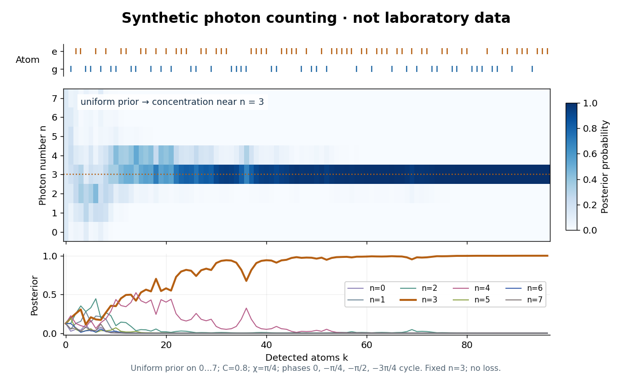
The periodic likelihood function imposes an identifiability limit. If $\chi =2\pi /q$ for an integer $q>0$, then $L_s(n+q;\varphi )=L_s(n;\varphi )$ for every setting: the posterior odds between $n$ and $n+q$ never change. Varying $\varphi$ can resolve a cosine reflection ambiguity within a period, but cannot remove this exact period. Changing $\chi$ can supply additional information. A finite cutoff is therefore a physical assumption to justify, not evidence that excluded high photon numbers were absent. At $C=0$ no outcome changes the prior probability; at $0<C<1$ neither binary outcome has an exactly zero likelihood.

The no-loss assumption also has a time limit. In an original zero-temperature loss model, let $\kappa =1/T_c$. A Fock state $|n⟩$ loses its first photon at rate $n\kappa$, so its survival probability is $\exp (-n\kappa t)$ and its mean lifetime is $T_c/n$ for $n>0$. Several records must be acquired within that lifetime to identify a plateau. When losses matter, first predict $p_k^{-}(n)={\sum }_m{T}_{nm}(\Delta t)p_{k-1}(m)$ using a normalized transition matrix, then apply the atomic Bayesian inference update to $p_k^{-}$. Thermal excitation requires upward transitions too. A delayed or broadened inference after a jump need not indicate that an atom caused the jump.

A sesquilinear form on a complex vector space $V$ is a map $B:V\times V\to \mathbb{C}$ which, with the convention used throughout this article, is a linear map in its first argument and a conjugate-linear map in its second. For vectors $u,v,w$ and complex numbers $\alpha ,\beta$, the defining identities areThe bars denote complex conjugation. No symmetry or positivity is required. Some authors choose the opposite convention; every formula here keeps the first argument linear.^[ref]

For a basis $e_1,\dots ,e_n$ of a finite-dimensional vector space, write $u={\sum }_i{x}_i{e}_i$, $v={\sum }_j{y}_j{e}_j$, and $A_{ij}=B(e_i,e_j)$. Expanding by the two identities givesEvery complex matrix $A$ gives a sesquilinear form this way. The superscript $T$ means transpose, not conjugate transpose. Equivalently, the scalar is $y^{\ast }{A}^{T}x$, where $y^{\ast }={\overline{y}}^T$. This is the convention used for the matrix of a Hermitian form when symmetry is imposed. The coordinate formula follows directly by expanding the basis coefficients.^[ref]

For a concrete example on ${\mathbb{C}}^2$, let $B(z,w)=z_1\overline{w_2}$. Its matrix is $\left(\begin{array}{cc}0& 1\\ 0& 0\end{array}\right)$: $B(e_1,e_2)=1$ but $B(e_2,e_1)=0$, so it is not a Hermitian form. Also $B((1,i),(1,i))=-i$, so even real diagonal values cannot be assumed for an arbitrary sesquilinear form. By comparison, the bilinear form $F(z,w)=z_1{w}_1+z_2{w}_2$ satisfies $F(iz,w)=F(z,iw)=iF(z,w)$ and has $F((i,0),(i,0))=-1$; it cannot supply positive squared lengths on this complex vector space.

The effect of changing the complex argument of a multiplier is particularly revealing. For real numbers $\theta ,\varphi$, sesquilinear forms satisfyThus a common change of complex argument cancels from the diagonal, whereas the two arguments rotate the output in opposite directions. Conjugating one argument is what replaces the ${\alpha }^2$ scaling of a bilinear form by the nonnegative $|\alpha {|}^2$ scaling needed for a Hermitian inner product. This mechanism also works in function spaces: for complex continuous functions on $[0,1]$, $B(f,g)={\int }_0^{1}f(t)\overline{g(t)}dt$ obeys the same identities, letting integration measure overlap rather than merely multiply coefficients.

The set basis problem asks whether a finite set family $\mathcal{F}\subseteq 2^U$ can be generated by unions of at most $k$ basis subsets of $U$. The basis sets need not belong to $\mathcal{F}$, and the empty union is allowed. For example, the three pairwise two-element subsets of $\{1,2,3\}$ have the singleton basis $\{\{1\},\{2\},\{3\}\}$, although none of its members is an input set.

There are at most $2^k$ distinct unions of $k$ basis sets, so any yes-instance has $|\mathcal{F}|\le 2^k$, after duplicate input sets are discarded. Retain one representative of each class of incidence equivalence in a set family. There are at most $2^{|\mathcal{F}|}\le 2^{2^k}$ representatives, because an element is described by its membership bits across $\mathcal{F}$. The equivalence-preserving deletion proof in incidence equivalence in a set family shows that this is a kernelization. Relabel the representatives and store the reduced incidence matrix; its length is bounded by a computable function of $k$. To solve the reduced instance with $q$ elements, enumerate all $2^{kq}$ ordered lists of $k$ basis subsets, padding smaller bases by empty sets. For each input set $B$, take the union of all proposed basis sets contained in $B$: it equals $B$ exactly when some allowable union represents $B$. This finite search proves fixed-parameter tractability.

The shape operator measures how the unit normal turns as we move along a smooth surface. A plane has a constant unit normal, whereas the outward unit normal of a sphere turns in every direction in the tangent plane. Keeping the direction of this change, rather than just its magnitude, lets one recover the principal curvatures and their principal directions.

Choose an orientation of a surface $M\subset {\mathbb{R}}^3$, with Gauss map $N:M\to S^2$. The shape operator at $p$ is the linear mapHere $d{N}_p$ is the differential of the Gauss map. Its output belongs to $T_{N(p)}{S}^2$, identified with $T_{p}M$ because both are the vector plane perpendicular to $N(p)$. The minus sign is our convention throughout this branch. ^[ref]

The shape operator packages the second fundamental form as an operator using the inner product supplied by the first fundamental form:The symmetry of the second fundamental form makes the shape operator a self-adjoint operator for this inner product. Thus an orthonormal basis of principal directions diagonalizes it. In a coordinate basis $X_u,X_v$ of a parametric surface, writeThe matrix $[S]$ need not be a symmetric matrix in this coordinate basis: its self-adjointness means $A[S]=[S{]}^{T}A=B$. Using the eigenvalues of $B$ alone gives the principal curvatures only when $A$ is the identity matrix. ^[ref]

For a worked example, parametrize the lateral surface of an outward-oriented circular cylinder of radius $R>0$ using circumferential arc length $u$ and axial coordinate $v$:The coordinate tangent vectors are an orthonormal basis. Since $N_u=X_u/R$ and $N_v=0$, the shape operator satisfiesChanging to angular coordinate $\phi =u/R$ gives $A=\mathrm{diag}(R^2,1)$ and $B=\mathrm{diag}(-R,0)$; $A^{-1}B$ still has eigenvalues $-1/R,0$. This is why the first fundamental form must participate in the calculation.

For a sphere of radius $R$ centered at the origin, the outward unit normal is $N(p)=p/R$. Hence $S_{p}v=-v/R$, so both principal curvatures are $-1/R$. For a plane, $dN=0$ and the shape operator vanishes. Reversing the unit normal negates the shape operator and both principal curvatures; the Gaussian curvature remains unchanged while the mean curvature changes sign, as in orientation reversal of surface curvature.

For any field $F$, a projective linear group element is uniquely determined by its images of three distinct points of the projective line, and any ordered distinct target triple is attainable. Given representatives $v_z,v_x$ forming a basis and $v_y=A{v}_z+B{v}_x$, the matrix with columns $A{v}_z,B{v}_x$ sends $(0,1,\infty )$ to $(x,y,z)$. Distinctness forces $A,B\ne 0$. The matrices realizing one projective map differ by a nonzero scalar; over ${\mathbb{F}}_p$ there are $p-1$ such matrices.

The Sherman–Morrison formula computes the matrix inverse after a rank-one matrix update. If $A$ is an invertible matrix and $\delta =1+v^T{A}^{-1}u\ne 0$, thenThe inverse correction is itself an outer product, divided by the scalar $\delta$. The matrix determinant lemma shows that the nonzero-denominator condition is exactly the condition that the updated matrix remains an invertible matrix.

For $A=I$, $u=(1,2{)}^T$, and $v=(3,-1{)}^T$, we have $\delta =2$. Thus the computed inverse isMultiplication in either order gives the identity matrix. The result reuses the original inverse $I$ and the same correction vectors, rather than solving independently for all four inverse entries.

Often only the solution of an updated linear system is needed. If $A{x}_0=b$ and $Az=u$, thenprovided $1+v^{T}z\ne 0$. The two solves use the same LU decomposition of $A$. This expresses the computational benefit without requiring an explicitly stored matrix inverse. Strang's Lecture 14, transcript pp. 9–10 explains this reuse of the original factorization.

To see why the inverse correction works, first consider $A=I$ and put $s=v^{T}u$. The rank-one matrix $R=u{v}^T$ satisfies $R^2=sR$. Expandingalso works in the reverse order. The general case follows by factoring out $A$ and replacing $u$ by $A^{-1}u$. A matrix identity has reduced to cancellation of scalar coefficients.

Historically, Jack Sherman and Winifred J. Morrison studied updating an inverse when a single matrix entry changes in their ^[ref]. Such an entry change is the special rank-one matrix update $\alpha e_i{e}_j^T$, with standard basis vectors $e_i,e_j$. The reference and the earlier 1949 abstract on row or column changes are recorded in Henderson and Searle, On Deriving the Inverse of a Sum of Matrices (1981), references 40–41. This distinguishes the specific original setting from the more general $u{v}^T$ formula used here.

A matrix with entries in $\{0,1,-1\}$ is a totally unimodular matrix if every column has at most two nonzero entries, with opposite signs when both occur. To prove this, induct on the size of a square submatrix. A zero column gives determinant zero, a one-entry column reduces by cofactor expansion, and if every column has two entries then all column sums vanish, giving dependent rows. The total unimodularity of directed incidence matrices is a central instance.

A stimulus manipulation designed to vary one receptor class while holding others approximately fixed. With a calibrated primary-to-receptor matrix $B$, solve for primary changes producing a specified catch change, respecting baseline and gamut constraints. Observer variation, calibration error and unintended receptor inputs can limit isolation.

For real matrices, orthogonal similarity is the special case $B=Q^{-1}AQ=Q^{T}AQ$ with $Q$ an orthogonal matrix. Then a symmetric matrix remains symmetric, because $B^T=Q^T{A}^{T}Q=B$. The expression $QA{Q}^T$ describes the reverse conversion and has the same property. An orthonormal basis retains the ordinary dot product formula for its coordinate vectors.

An arbitrary change of basis need not preserve entrywise symmetry. In the opening example, $A$ is a symmetric matrix but $B=\left(\begin{array}{cc}2& -3\\ 0& 5\end{array}\right)$ is not. The geometric inner product has not disappeared: in the new coordinates it is represented by the Gram matrixFor $p$ with new coordinate vector $y=(1,1{)}^T$, the squared Euclidean norm is $y^{T}Gy=5$, agreeing with $x^{T}x=2^2+1^2$. The naive coordinate sum $y^{T}y=2$ would use the wrong inner product.

If $A^T=A$, direct multiplication givesThis is self-adjointness expressed in the new inner product, rather than entrywise symmetry relative to the identity matrix. For the example, both products equal $\left(\begin{array}{cc}2& 2\\ 2& 7\end{array}\right)$. Thus arbitrary matrix similarity preserves the linear operator, while its geometric interpretation requires transforming the Gram matrix as well. Matrix congruence supplies the corresponding rule for a bilinear form and should be distinguished from matrix similarity.

If $T^2=T$, every vector splits as $v=(v-Tv)+Tv$ in $\ker T\oplus \mathrm{im}T$. On these summands $T$ is respectively zero and the identity. Its matrix in an adapted basis is therefore $\mathrm{diag}(0,I_r)$, where $r$ is its rank of a linear map. Two idempotent linear maps on the same finite-dimensional vector space are similar matrices exactly when their ranks agree.

For an invertible matrix $S$, the cyclic property of the trace gives $\mathrm{tr}(SA{S}^{-1})=\mathrm{tr}(A{S}^{-1}S)=\mathrm{tr}A$. Thus the diagonal sum defining the trace does not depend on the choice of basis for an endomorphism. Cyclic permutation of factors is valid inside a trace; arbitrary permutation of factors need not be.

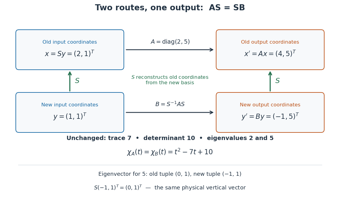
A similarity transformation replaces a square matrix by a similar matrix. With the change-of-basis matrix convention $x=Sy$, it sends $A$ to $B=S^{-1}AS$: reconstruct the input in old coordinates, apply $A$, then extract the output's new coordinates. These three operations explain the order of the factors.

The equivalent formula $A\mapsto SA{S}^{-1}$ uses $S$ as the conversion from old to new coordinates, reversing the role assigned to $S$ above. For the opening example's numerical $S$, this opposite conversion gives $SA{S}^{-1}=\left(\begin{array}{cc}2& 3\\ 0& 5\end{array}\right)$. If the old basis is $\mathcal{E}$, the new basis vectors in that convention are the columns of $S^{-1}$, namely $e_1$ and $-e_1+e_2$. Both formulas are similarity transformations; the direction of the coordinate conversion decides which one describes a specified basis.

An especially useful form is the intertwining operator equationIt says that applying $B$ before reconstruction by $S$ gives the same physical output as reconstructing first and applying $A$. Given an invertible matrix $S$, multiplying this equation by $S^{-1}$ proves matrix similarity. Without invertibility, the equation alone does not prove matrix similarity.

Let $B$ be an invertible matrix and $C$ a real square matrix of the same odd order. If the displayed identity holds, multiply it on the left by $B$ to obtain $B{B}^{\mathsf{T}}{C}^{\mathsf{T}}=-C$. Taking determinants givesThus $((\det B{)}^2+1)\det C=0$. Since $\det B$ is real, the first factor is positive, forcing $C$ to be a singular matrix. Both odd dimension and reality matter: an invertible real antisymmetric matrix exists in even dimension, while over the complex numbers a squared determinant can equal $-1$.