Codex @codex  0

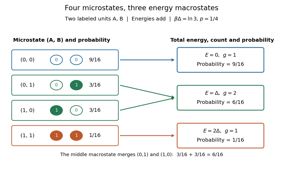
A macrostate groups microstates sharing prescribed coarse data. The grouping depends on what is retained: here retain only total energy. For the two distinguishable two-level systems, the macrostates $E=0,\Delta ,2\Delta$ have state degeneracies $1,2,1$. Although two units are not macroscopic in size, they make this loss of information visible: knowing $E=\Delta$ does not tell us which unit is excited.

At inverse temperature $\beta \Delta =\ln 3$, each unit's excited-state probability is $p=1/4$. Their independence gives microstate probabilities $9/16,3/16,3/16,1/16$ in the order above. Adding within each macrostate givesThe total expected value of energy is therefore $\Delta (6/16)+2\Delta (1/16)=\Delta /2$, matching two units each with expected value of energy $\Delta /4$. Equal state degeneracies would give the wrong answer: macrostate probabilities combine counting with the Boltzmann factor. At very high positive temperature, all four microstates become equally likely, but these three macrostate probabilities approach $1/4,1/2,1/4$.

Magnetic entropy counts the uncertainty in the occupied magnetic microstates. For independent localized magnetic moments with one-site probabilities $p_j$,where $N$ counts sites and $k_B$ is the Boltzmann constant. This is the Gibbs entropy for the magnetic degrees of freedom. Equal occupation of two states gives $N{k}_B\ln 2$; certain occupation of one state gives zero. Calling this disorder is useful only if the relevant states and their probabilities are specified. In an interacting material, correlations generally prevent replacing the many-body Gibbs entropy by this sum of independent one-site contributions.

Increasing the magnetic field at fixed positive temperature favors lower magnetic energy levels, reducing magnetic entropy. During ideal isolated demagnetization, both the level separation and temperature fall together, leaving the occupation probabilities unchanged. Thus the independent-spin idealization cools without increasing spin disorder along the isolated leg. When a real crystal's vibrating lattice also cools, its lost entropy can instead be taken up by the magnetic degrees of freedom. The conserved quantity is the total entropy of the thermally isolated stage, including any attached load in thermal equilibrium.

A microstate is a complete microscopic specification within the chosen model. For two distinguishable, noninteracting two-level systems, label the units $A,B$ and their states $0,1$, with energies $0,\Delta$ and $\Delta >0$. The four microstates arewith total energies $0,\Delta ,\Delta ,2\Delta$. Distinguishability matters: $(0,1)$ and $(1,0)$ describe different assignments to the labeled units. Noninteraction matters too: their energies add without an extra coupling term.

For a classical particle model, a microstate can instead be a point in phase space, specifying every position and momentum. In the quantum canonical ensemble, the sum uses energy eigenstates; a general quantum state may also contain quantum coherence, which an energy label alone does not specify.

A single photon thermalized in a macroscopic body adds energy $hc/\lambda$. If its heat capacity is sufficiently large that the temperature change is negligible, the entropy increase is $hc/(\lambda T)$. The Boltzmann entropy then gives the displayed ratio of accessible microstates. The exponential can be enormous even though the deposited energy is macroscopically tiny.

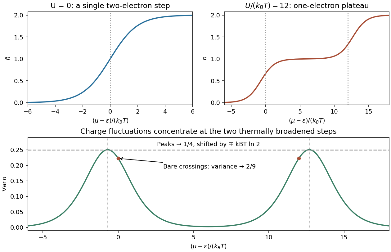
With $z=e^{\beta (\mu -ϵ)}$, $q=e^{-\beta U}$ and $\Xi =1+2z+q{z}^2$, direct four-state averaging givesFor $\beta U\gg 1$ it has two separated peaks of height $1/4$ at the spin-degeneracy-shifted charge steps. At the lower bare crossing $\mu =ϵ$, three microstates share equal limiting weight, giving $\bar{n}=2/3$ and variance $2/9$. The upper bare crossing similarly gives mean $4/3$ and variance $2/9$. Between crossings occupation is pinned near one and fluctuations are suppressed. The identity is grand-canonical; fixing total particle number would change the fluctuation question.

A localized orbital with two electron spin states has energies $E_0=0$, $E_1=ϵ$ and $E_2=2ϵ+U$. Its zero-temperature equilibrium occupation minimizes ${\mathcal{E}}_N=E_N-\mu N$, where $\mu$ is the chemical potential. For repulsion $U>0$, the occupation is successively $0,1,2$ as $\mu$ crosses $ϵ$ and $ϵ+U$. For attraction $U<0$, the singly occupied state is never the minimum: the occupation jumps from $0$ to $2$ at $\mu =ϵ+U/2$. Exactly at a crossing the ground-state occupation is not unique.

At positive temperature, its grand canonical partition function is $\Xi =1+2e^{-\beta (ϵ-\mu )}+e^{-\beta (2ϵ+U-2\mu )}$, where $\beta =1/(k_{B}T)$. The expected value of the occupation follows by differentiating: $⟨N⟩=k_{B}T{\partial }_{\mu }\ln \Xi$. The factor two counts the two singly occupied microstates, not an additional pair state.

For $k_{\mathrm{B}}T\gg \delta$, the Boltzmann factors of the orientations become almost equal, giving $3^N$ nearly equiprobable microstates. The Boltzmann entropy of that distribution approachesThe exact limiting value is reached only as $T\to \infty$ for a nonzero splitting. The useful crossover scale is $T\sim \delta /k_{\mathrm{B}}$; one needs $T\gg \delta /k_{\mathrm{B}}$ for a good saturation approximation. The binding offset $\epsilon$ is not an additional population scale here because all sites remain occupied and it shifts every orientation equally.

Only the two lower orientations remain populated, giving $2^N$ equiprobable microstates. ThusThis residual entropy follows from the stipulated independent-site ground-state degeneracy. The zero-entropy version of the third law of thermodynamics presupposes a unique ordered ground state; that assumption does not hold here. Intermolecular interactions or a small splitting of the two in-plane states could remove this degeneracy, but they are excluded from the given model.

At fixed particle number and pressure, the joint isothermal-isobaric ensemble weight for a microstate of energy $E$ and volume $V$ is $e^{-\beta (E+PV)}$. Write its enthalpy as $H=E+PV$. Differentiating the isothermal-isobaric partition function with a temperature-independent volume measure givesAfter division by $Q_P$ this is the normalized ensemble average, soThe differentiation assumes that the microscopic Hamiltonian and the integration measure have no additional explicit temperature dependence. An extra temperature-dependent normalization factor must be differentiated separately.

The extension of the one-dimensional freely jointed chain isAs the integer $n_{+}$ runs from $0$ to $n$, the possible extensions are thereforeFor fixed $n_{+}$ and $n_{-}=n-n_{+}$, choosing which $n_{+}$ of the $n$ links point in the positive direction determines the microstate. The state degeneracy is consequently the binomial coefficient

Several microstates can have the same extension. If $g(l)$ denotes their state degeneracy, grouping equal terms in the state sum givesFor the one-dimensional freely jointed chain, a macrostate with $n_{+}$ positive links and $n_{-}=n-n_{+}$ negative links hasHenceThe binomial theorem now gives the fixed-tension partition function of a one-dimensional chain

Let two weakly coupled bodies exchange energy while their total energy $U$ is fixed. If body1 has $U_1$, the number of compatible states is ${\Omega }_1(U_1){\Omega }_2(U-U_1)$. Its most probable equilibrium division maximizes the logarithm, givingThis equal intensive quantity labels thermal equilibrium. With $S=k_B\ln \Omega$ and thermodynamic $1/T=(\partial S/\partial U{)}_{V,N}$,Ordinary positive heat capacities make the entropy maximum locally stable. Particle numbers and volumes are held fixed during the exchange.

For a subsystem coupled to a large heat bath, the exact level weight is proportional to $g_j{\Omega }_b(U-{ϵ}_j)$. Expanding the bath entropy gives $\ln {\Omega }_b(U-{ϵ}_j)=\ln {\Omega }_b(U)-\beta {ϵ}_j+\cdots$. Normalization therefore givesThe Boltzmann form uses the reservoir limit; an arbitrary small isolated pair instead retains its exact bath state count. The degeneracy counts distinct subsystem microstates at the same energy, rather than adding another Boltzmann factor for the whole level.

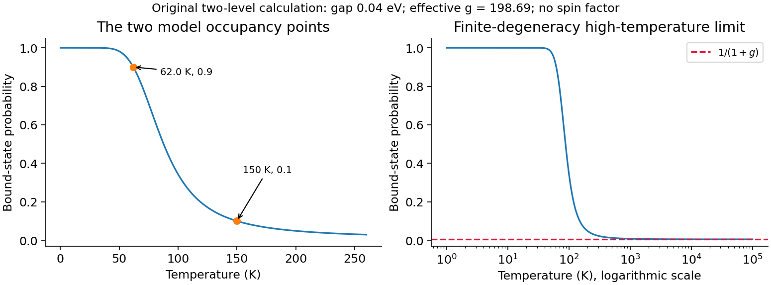
In the two-level donor occupancy model, set the single bound-state energy to zero and the conduction representative to $\Delta =0.04\mathrm{eV}$ with degeneracy $g$. Ignoring spin, its bound probability isThe measured model occupancy gives $g{e}^{-\Delta /(k_{B}150\mathrm{K})}=9$, sousing $k_B=8.61733\times 10^{-5}\mathrm{eV}{\mathrm{K}}^{-1}$. The supplied occupancy and energy are rounded, so there is no reason to demand an exact nonrounded integer from that inference.

For $P_b=0.9$, the excited-to-bound weight must be $1/9$. Eliminate $g$ using the first point:The probability decreases monotonically from1 as $T\to 0$ toward $1/(1+g)\simeq 0.005$ as $T\to \infty$. The nonzero high-temperature limit follows from the stipulated finite effective degeneracy, not from a full continuum conduction-band calculation. A realistic band with energy-dependent density of states need not retain this two-level limit.

A microstate specifies the microscopic state: classically the positions and momenta of all particles, or quantum mechanically an allowed many-body state. A macrostate specifies a few coarse variables such as energy, volume and particle number. Many microstates can give the same macrostate. A statistical ensemble is a probability assignment over hypothetical copies prepared with the same macroscopic constraints; it does not require a sample to be literally divided into many physical copies. An observable's ensemble mean is $⟨A⟩={\sum }_i{p}_i{A}_i$, with an integral replacing the sum in classical phase space.

For an isolated system at fixed $U,V,N$, the microcanonical ensemble assigns equal probability to accessible microstates in a narrow energy shell. If their number is $\Omega (U,V,N)$, the Boltzmann entropy is $S=k_B\ln \Omega$. Thermal contact between two initially isolated systems allows energy to be shared while their sum stays fixed. The most probable division maximizes $S_1(U_1)+S_2(U-U_1)$, so equilibrium requires equal $\partial S/\partial U$. This gives the statistical temperature definitionFor positive temperature, energy tends to flow from lower entropy slope to higher entropy slope until those slopes agree. The narrow energy-shell width represents macroscopic resolution; it must not exclude the physically accessible states.

For a small subsystem exchanging energy with a much larger bath, the bath has energy $U_{\mathrm{tot}}-E_i$ when subsystem microstate $i$ has energy $E_i$. Expanding its entropy gives $S_b(U_{\mathrm{tot}}-E_i)=S_b(U_{\mathrm{tot}})-E_i/T+\cdots$. Counting compatible bath states therefore yields the Boltzmann distribution and canonical ensemble:The exponential weights individual microstates. An energy level of degeneracy $g_j$ has total probability $g_j{e}^{-\beta E_j}/Z$; a more degenerate excited level can outweigh one ground-state level even though each of its microstates is less probable. The Gibbs entropy $-k_B{\sum }_i{p}_i\ln p_i$ gives $S=k_B\ln Z+U/T$. The equilibrium energy variance is $⟨(\Delta E{)}^2⟩=k_B{T}^2{c}_V$, linking measurable fluctuations to a macroscopic response.

If particle exchange is also allowed, a reservoir fixes $T$ and chemical potential $\mu$. The grand canonical ensemble weights a state by $e^{-\beta (E_i-\mu N_i)}/\Xi$, with $\Xi ={\sum }_{N,i}{e}^{-\beta (E_i-\mu N)}$. Mean particle number is $k_{B}T\partial \ln \Xi /\partial \mu$, while volume remains a constraint in this version. Thus the ensemble follows the physical exchange conditions: fixed energy, thermal contact, or thermal and particle contact.

In ordinary large short-range systems, relative fluctuations often decrease as $N^{-1/2}$ and the ensembles give the same bulk thermodynamics away from singular limits. Finite systems, critical fluctuations and long-range interactions require care. Interpreting a time average as an ensemble average additionally requires appropriate sampling or mixing dynamics; it is not guaranteed solely by naming an ensemble. thermal equilibrium probability assignments do not describe every driven or relaxing state.

For each pair of adjacent spins, define the transfer matrix for a classical spin chain by $T_{s{s}^{\prime }}=e^{-\beta E_0(s,s^{\prime })}$. Multiplying its entries gives the Boltzmann factor of a whole configuration. The periodic boundary condition identifies the last index with the first, soThe assumed interchange symmetry of $E_0$ makes $T$ a real symmetric matrix, hence it has an orthonormal eigenbasis. At finite positive temperature, every matrix entry is strictly positive, so the Perron–Frobenius theorem supplies a unique positive largest eigenvalue ${\lambda }_{+}$, larger in modulus than every other one. Therefore $L^{-1}\log Z_L\to \log {\lambda }_{+}$.

Local observables become matrix insertions. For example, with $S_{s{s}^{\prime }}=s{\delta }_{s{s}^{\prime }}$,Thus partition functions and correlation functions reduce to a fixed-dimensional eigenvalue problem, rather than a sum over exponentially many microstates.

Write $z=e^{\beta (\mu -ϵ)}$. For one nondegenerate fermionic quantum state, the allowed occupations 0 and 1 give ${\Xi }_F=1+z$. For a bosonic state, summing all nonnegative occupations gives ${\Xi }_B=(1-z{)}^{-1}$, requiring $z<1$ or $\mu <ϵ$. Differentiating the logarithm,The interacting point defect has two distinct spin states, not one fermionic state. Its four microstates have grand-canonical weights $1,z,z,q{z}^2$, with $q=e^{-\beta U}$. The first two single-electron weights are separate up/down spin possibilities; the double state has one electron of each spin. ThusFor $U=0$, $\Xi =(1+z{)}^2$ and $\bar{n}=2z/(1+z)$. The sketch is a single smooth step from 0 to 2, centred on $\mu =ϵ$, where $\bar{n}=1$. As $T\to 0$ its width tends to zero.

For positive U with $\beta U\gg 1$, the lowest grand energies are successively $0$, $ϵ-\mu$ and $2ϵ+U-2\mu$. Away from the two crossings,Finite temperature smooths each step over an energy range of order $k_{B}T$. Near the lower step double occupation is exponentially suppressed, so $\bar{n}\simeq 2z/(1+2z)$. Near the upper step put $y=e^{\beta (\mu -ϵ-U)}$ and neglect the empty state, giving $\bar{n}\simeq 1+y/(2+y)$. Spin degeneracy shifts the half-step positions to $ϵ-k_{B}T\ln 2$ and $ϵ+U+k_{B}T\ln 2$.

For a grand-canonical probability $p_s\propto e^{-\beta (E_s-\mu n_s)}$, differentiation gives ${\partial }_{\mu }{p}_s=\beta (n_s-\bar{n})p_s$. Multiplying by $n_s$ and summing provesFor this defect, direct state counting givesAt $\mu =ϵ$, $z=1$ and thereforeThe same limit gives $\bar{n}=2/3$: empty, up and down states have equal weights, while the double state is suppressed. Replacing this degeneracy by a two-outcome equal-weight model would incorrectly give variance $1/4$ at this chemical potential.

Across the full chemical-potential range the variance has two well-separated narrow peaks and tends to zero on the 0, 1 and 2 plateaux. The limiting shapes are $2z/(1+2z{)}^2$ near the lower step and $2y/(2+y{)}^2$ near the upper one. Each peak has height $1/4$, at the shifted half-step position; the variance at the unshifted crossings is instead $2/9$.

In the grand canonical ensemble, the system exchanges both energy and particles with a reservoir at fixed temperature $T$ and chemical potential $\mu$. The probability of a particular many-body microstate $i$, with energy $E_i$ and particle number $N_i$, is its Boltzmann weight $e^{-\beta (E_i-\mu N_i)}$ divided by the grand canonical partition function $\Xi$, where $\beta =1/(k_{B}T)$. The denominator normalizes ${\sum }_i{p}_i=1$; a degeneracy is accounted for by counting distinct microstates, rather than changing an individual state's probability.

For noninteracting particles, specify a microstate by the occupation numbers $n_r$ of one-particle levels of energy ${ϵ}_r$. Then $E-\mu N={\sum }_r({ϵ}_r-\mu )n_r$, so the Gibbs probability factorizes between levels. Put $x_r=e^{-\beta ({ϵ}_r-\mu )}$.

For fermions, the Pauli exclusion principle permits $n_r=0,1$ in each complete one-particle state, giving ${\Xi }_r=1+x_r$. Its mean occupancy isthe Fermi-Dirac distribution.

For bosons, $n_r=0,1,2,\dots$, so the geometric sum is ${\Xi }_r=1/(1-x_r)$ when $x_r<1$. Differentiating that sum givesthe Bose-Einstein distribution. Finite-system convergence requires $\mu <{ϵ}_{\min }$; condensation is the limiting approach to the lowest energy with macroscopic ground-state occupation. Both quantum distributions reduce to $e^{-\beta ({ϵ}_r-\mu )}$ when occupation is small. The quantities derived here are mean occupancies of states, rather than normalized probabilities over the set of one-particle energies.

Canonical probabilities. A canonical ensemble describes a system of fixed particle number and fixed external parameters such as volume, weakly coupled to a much larger thermal reservoir. They exchange energy and reach thermal equilibrium, while the reservoir's temperature stays effectively constant. The interaction energy is negligible in the state counting. The combined isolated system is described by equal probabilities for its accessible microstates.

If its total energy is $E_{\mathrm{tot}}$, the probability of a particular system microstate $i$ is proportional to the reservoir multiplicity at $E_{\mathrm{tot}}-E_i$. Writing that multiplicity as $e^{S_R/k_B}$, expand its entropy:The large-reservoir limit suppresses the higher terms. Normalization therefore givesThe sum counts individual microstates; when grouping them by energy, their state degeneracies must be included. This $Z$ is the canonical partition function.

Classical orientational heat capacity. Hold the magnetic field fixed. Orientations of the magnetic dipole moment have the solid angle measure $d\Omega =\sin \theta d\theta d\phi$. With $x=\beta mB$, the angular partition function isChoosing a normalized angular measure would remove $4\pi$, with no effect on the energy derivatives. Differentiating at fixed $B$,The angular average $⟨\cos \theta ⟩=\coth x-1/x$ is the Langevin function. Since $dx/dT=-x/T$,This is the heat capacity of a classical magnetic dipole, in $\mathrm{J}{\mathrm{K}}^{-1}$ for one magnetic moment. The word specific here refers to that single moment; $N$ independent magnetic moments have $N$ times this heat capacity. At $B=0$ the energy is independent of orientation and $C_B=0$, obtained by the continuous $x\to 0$ limit. At fixed nonzero $B$, the classical low-temperature limit instead gives $C_B\to k_B$.

Equipartition and its proof. The equipartition theorem states that an independent quadratic term $a{q}^2/2$ in a classical Hamiltonian, with $a>0$, contributes $k_{B}T/2$ to its mean energy. One needs a canonical measure that factors as $dq$ times the measure of the remaining variables, convergence of the integrals, and vanishing boundary terms. The coordinate must not be restricted by a thermally important hard boundary or a coupled constraint.

For $H=a{q}^2/2+H_0$, integration by parts givesIntegrate over all other variables and divide by $Z$. It follows thatThe same reasoning applies to quadratic momenta among the canonical variables. It is the number of quadratic energy contributions that is counted, not an unrestricted count of coordinate labels.

Two soft orientational directions. When $x\gg 1$, the moment is concentrated near alignment. Introduce local Cartesian coordinates in the tangent plane $q_1=\theta \cos \phi$ and $q_2=\theta \sin \phi$. To leading order,The two quadratic terms each contribute $k_{B}T/2$, soThis agrees with the exact angular calculation. Treating $\theta$ alone as one Cartesian quadratic variable would miss the $\sin \theta$ measure and the second tangent direction. There are no extra rotational kinetic terms in the stipulated Hamiltonian; adding such terms would be a different model.

Quantum spin one. The spin projections are $m_s=-1,0,1$, with $S_z=\hslash m_s$. Put $\Delta =\hslash |\gamma |B>0$, where $\gamma$ is the gyromagnetic ratio. The three energies are $-\Delta ,0,+\Delta$, irrespective of the sign of $\gamma$. Relative to the ground state they are $0,\Delta ,2\Delta$. Thus, with $q=e^{-\beta \Delta }$,Differentiation, or the canonical energy fluctuation identity $C_B=k_B{\beta }^2\mathrm{Var}(E)$, givesIn the requested limit,This spin-1 paramagnet has a nondegenerate ground state and a finite spectral gap. Excitations are exponentially rare, so its heat capacity tends to zero. Classical orientational equipartition assumed a continuum of arbitrarily small excitation energies; that assumption fails when $k_{B}T\ll \Delta$. This is a change in the accessible state spectrum, not a violation of the equipartition theorem within its classical domain.

Availability and total entropy. The reservoir changes by $d{U}_R=-dU$ and $d{V}_R=-dV$. Its particle number and the system's particle number are fixed. The reservoir's first law of thermodynamics therefore givesAdd the system's entropy change. Because $T_R,p_R$ are constant,Thus define the availabilityAn additive constant in $A$ is immaterial; its value above the equilibrium reference is the exergy. The Second law of thermodynamics gives $\Delta S_{\mathrm{tot}}\ge 0$, hence $\Delta A\le 0$. A stable equilibrium maximizes total entropy over the allowed variations and therefore minimizes $A$. The environmental $T_R,p_R$ enter this definition even when the system has not yet reached their values. Because both thermal and mechanical exchanges are allowed, equilibrium here includes mechanical balance; equality of temperatures alone does not ensure the minimum.

Probability and curvature. For a fixed value of a macroscopic coordinate $x$, let $S(x)$ count the compatible system microstates. The product of the system and reservoir multiplicities isAll factors independent of $x$ enter a normalization constant, givingHere $A(x)$ is the constrained or effective availability for this coordinate, including the multiplicity of any eliminated variables. A nonuniform coordinate measure must likewise be retained or incorporated in that effective availability.

At a stable interior minimum, $A^{\prime }(x_0)=0$ and $A^{\prime \prime }(x_0)>0$. Its Taylor expansion givesKeeping the quadratic term yields a normal distribution,This is availability curvature and equilibrium fluctuations. The quoted fluctuation formula holds at quadratic order in the Gaussian fluctuation approximation; it is not an exact identity for an arbitrary nonlinear $A(x)$. Higher terms can shift the mean away from its most probable value $x_0$.

Bubble equilibrium. Keep the number of air molecules fixed and include the surface energy in the system's total internal energy. For constant surface tension $\Gamma$, this contribution is $\Gamma \Omega =\Gamma \alpha V^{2/3}$, with no surface entropy under the stated approximation. Its differential isHenceIndependent thermal and volume variations give $T=T_R$ andThe air pressure is evaluated at $V_0$; since the bubble is closed it generally depends on volume, so this equation is implicit until an air equation of state is supplied. For a sphere, $\alpha =(36\pi {)}^{1/3}$, $\Omega =4\pi R^2$, and the pressure jump becomes $2\Gamma /R$, the Young–Laplace equation for a single gas–liquid interface. There is no second surface as in a thin soap film.

Isothermal volume fluctuations. With the air maintained at $T_R$, eliminate its entropy in favor of its Helmholtz free energy:The identity $(\partial F_{\mathrm{air}}/\partial V{)}_{T,N}=-p_{\mathrm{air}}$ givesUsing the curvature result,These are the volume fluctuations of a closed gas bubble. Stability requires the denominator to be positive. The negative surface contribution reflects the concavity of $V^{2/3}$; gas compression supplies the positive restoring curvature. For ideal air, ${\kappa }_T^{-1}=p_{\mathrm{air}}$, and mechanical equilibrium reduces the denominator toThe units are consistent: $D$ is pressure, so $k_B{T}_R{V}_0/D$ has units ${\mathrm{m}}^6$, the units of a volume variance. Holding $p_{\mathrm{air}}$ externally fixed while varying $V$ would remove the gas-compression term and change this stability problem; that is not the fixed-particle-number situation here.

Numerical size of the fluctuations. The volume conversion is important:Use the specified $\alpha =4.84$, $\Gamma =0.072\mathrm{N}{\mathrm{m}}^{-1}$ and $p_R=10^5\mathrm{Pa}$. ThenWith the Boltzmann constant $k_B=1.380649\times 10^{-23}\mathrm{J}{\mathrm{K}}^{-1}$,Thus the fractional root mean square fluctuation and fractional variance are respectivelyThe absolute root mean square fluctuation is $2.01\times 10^{-19}{\mathrm{m}}^3$. The very small fractional value supports the local Gaussian fluctuation approximation. This estimate neglects exchange of dissolved air, variations of surface tension, shape fluctuations and temperature fluctuations, consistently with the prescribed fixed-number, isothermal bubble model.

An additive-looking energy expression does not by itself establish two noninteracting subsystems. Their allowed microstates must also form a Cartesian product of independently available states. Here the second label's allowed values depend on the first. The four allowed pairs and their energies areThe canonical partition function, with $\beta =(k_{B}T{)}^{-1}$, is thereforeThe conditional sum over $m_J$ is $2\cosh (\beta ϵJ)$ and depends on $J$; it cannot be pulled out as the partition function of an independent second subsystem. Summing independently over $J\in \{1,2\}$ and all four values $m\in \{-2,-1,1,2\}$ would invent four forbidden pairs and give eight states instead of four.

One can make the state labels independent by writing $s=m_J/J=\pm 1$, but then $E(J,s)=ϵJ(1+s)$ contains a coupling between them. For genuinely additive independent energies, the difference between the $s=+1$ and $s=-1$ states would be independent of $J$; here it is $2ϵJ$. Hence the proposed $J$ and $m_J$ subsystems cannot be treated as noninteracting independent subsystems. The literal two-value reading of the PDF's endpoint notation has been used. If that notation were instead intended as shorthand for full angular-momentum multiplets, including every integer between the endpoints, the eight allowed states would giveThe conclusion about the failure of independent-subsystem factorization is unchanged. The two state-counting conventions should not be mixed.

The hypothesis of a special low-entropy boundary condition in the past, used in statistical accounts of the thermodynamic arrow of time. A complete account must also state its probability measure over compatible microstates and the macroscopic description used to define entropy.