De Moivre's theorem says that, for a real angle and an integer ,For a complex number , the corresponding formula is , with required for negative powers.
Put . If , the finite geometric series givesTo extract the real part, multiply numerator and denominator by . The denominator becomes , and the numerator is . Thus this finite trigonometric sum isAt , the sum equals ; the printed quotient is undefined there, though its continuous limiting value is .
Taking the conjugate transpose of and using that both parts are Hermitian matrices gives . Addition and subtraction recover the Hermitian parts of a unitary matrix:These depend only on , so any such decomposition has the same and is unique. Conversely the displayed expressions are Hermitian matrices and sum to in the form , establishing existence as well as uniqueness. Their commutation and quadratic relation are proved in the two labelled parts.
By the unitary matrix identities,Subtracting the two equations yields . ThereforeThe subtraction is important: entrywise real and imaginary parts cannot generally be used to separate these terms, since the Hermitian matrices need not have real entries.
Adding the two expanded unitary matrix identities instead cancels the commutator and gives . HenceTogether with part (i), this characterizes the commuting Hermitian parts of a unitary matrix.
The ratio test states that, for a series with nonzero terms eventually, if , the series converges absolutely; if , including , it diverges because its terms do not tend to zero. At the test is inconclusive: the harmonic series diverges while converges.
For , the ratio test applied to gives absolute convergence when , and at every such term vanishes. ThusAt all terms are zero, so the series converges to zero. At , the even terms vanish and the odd terms are , whose partial sums tend to . Finally, if , then , so the term test for divergence applies. Consequently
Fix . For any sufficiently small nonzero , the additivity of the Riemann integral givesTaking absolute values, for either sign of ,Because is continuous at , the right side tends to zero. Thus the fundamental theorem of calculus here follows directly from the difference quotient:Only continuity at the point under consideration was used.
Without continuity, the assertion is false. Take the Riemann integrable step function for and for . Its primitive is for and for . The left and right difference quotients at are respectively zero and one, so the primitive need not be differentiable at every interior point. A function with this single jump is Riemann integrable; changing its value at the jump does not change the integral or the counterexample.
In suffix notation, repeated indices are summed from one to three. The Levi-Civita symbol and Kronecker delta contraction isFor distinct free index pairs this follows from the two possible matching permutations and their signs; if either pair repeats an index both sides vanish. ThereforeRecognizing the dot products proves the vector triple product identity:
Use the Levi-Civita symbol contraction in suffix notation:Thus the cross product contraction expands as
Put . The vector triple product identity givesCyclic invariance of the scalar triple product gives . Hence the squared scalar triple product from cyclic cross products isIf an expansion entirely in pairwise dot products is desired, expand the Gram determinant of :Both expressions remain valid for degenerate, including linearly dependent, vectors.
The parametric equation of a straight line through with unit direction isIf the two lines meet, then for some real , so lies in the linear span of their direction vectors. Its dot product with their cross product is consequently zero:This is not sufficient without excluding parallel lines. For instance , and satisfy it, but the lines are distinct and never meet. For nonparallel lines the condition is sufficient, because the two directions span the plane perpendicular to their nonzero cross product.
For nonparallel skew lines, put . Every joining vector is , with fixed component along . Its length is at least the absolute value of that component. Its perpendicular component can be canceled by a unique choice of , since the two independent directions span . This lower bound is attained, proving the distance between skew lines:
For two upper triangular matrices and ,Indeed a potentially nonzero factor requires , while a potentially nonzero requires . These requirements cannot both hold when . Thus their matrix product is upper triangular.
Direct matrix multiplication for the given givesAdding yields , so . HenceEvery nonnegative matrix power is in : reduce powers of degree at least three using . More formally, repeated reduction shows that products of any two polynomials of degree at most two in again lie in this span. Since also lies in it, positive powers of prove the same assertion for all negative integers. This is an instance of the integer powers for an annihilating polynomial with roots one and minus one, because .
To find the required entries for every integer, use the block upper-triangular structure. The top-left entry of is for positive and negative powers. Its lower-right block isThe identity holds for all integers: multiplication adds the coefficients of , and proves the negative cases. ThereforeWrite and . Comparing those three entries givesSubtracting the first two equations finds ; the third then finds , and the first finds . The unique solution isFor clarity, substituting also gives the full matrix power
If are orthonormal, any relation gives on taking the dot product with . Thus the vectors are linearly independent. A linearly independent set of vectors in the -dimensional vector space is a basis, proving the claim.
Expand both and in this orthonormal basis, writing . Since , the linear equation becomesComparing the unique basis coefficients gives, when is not an eigenvalue,If , the equation is solvable exactly when for every with . For those indices is arbitrary; for all other indices the displayed formula still applies. Thus repeated eigenvalues require orthogonality to the entire corresponding eigenspace, not merely to one chosen eigenvector. This is the finite-dimensional Fredholm solvability condition for a self-adjoint operator.
For the specific real symmetric matrix, chooseTheir dot products with are , and . At this givesOne can check directly. At , the first coefficient equation would require , which is impossible. Hence there is no solution when ; the nonzero projection onto its eigenspace is the obstruction.
Let be a Hermitian matrix and with . The inner product is real because its conjugate equals . But it also equals , with . Thus every eigenvalue is real. For two eigenvectors,When , this proves , so the eigenvectors are orthogonal.
For a real antisymmetric matrix, , so is a Hermitian matrix. Its real eigenvalues imply that the eigenvalues of are purely imaginary. To ensure a nonzero one without assuming it, writeExpansion of the characteristic polynomial gives . Therefore the nonzero eigenvalue exists with , and a nonzero complex eigenvector satisfiesSeparating real and imaginary parts givesNeither real vector can vanish, since either vanishing would force the other to vanish. Antisymmetry yields andThus are orthogonal and have equal length.
In odd dimension , so . Its real homogeneous system therefore has a nonzero real eigenvector with . It is perpendicular to , because and similarly for . Normalize it and choose its sign so is positively oriented; this is an orthonormal basis.
The matrix exponential series converges absolutely, allowing even and odd terms to be grouped. Since and , it acts asConsequently the skew-symmetric exponential as an axial rotation has, in the displayed orthonormal basis, the matrixIt is orthogonal with determinant one, fixes its axis and rotates the perpendicular plane. Hence is a rotation matrix, with angle about the chosen oriented axis.
The comparison test for series says that an eventual upper bound by a convergent positive series proves convergence, while an eventual lower bound by a divergent positive series proves divergence. The p-series converges exactly when .
If , then for all sufficiently large , soand the series converges. If , choose . The allowed logarithmic bound, applied with exponent , gives eventually. Thusand the series diverges.
For , use the integral test for convergence: for an eventually positive decreasing function , and either both converge or both diverge. Here is decreasing for , and the substitution givesThis integral converges exactly when . Hence the polynomial-logarithmic series convergence classification isAll other allowed positive give divergence.
For any fixed , as . For example, l'Hôpital's rule applied to gives the limit zero. With , this implies eventually. Thereforefor all sufficiently large . The comparison series diverges by the integral test for convergence, sinceThe comparison test for series givesOne may obtain the same growth bound by extending the given logarithmic estimate to real through and choosing any exponent smaller than ; no special convergence test for iterated logarithms is needed.
The intermediate value theorem states that, if is a continuous function on a closed interval , every value between and equals for some . If the value is strictly between the endpoint values, may be chosen in .
Here is a proof from the supremum property of the real numbers. Suppose ; the reverse inequality is reduced to this case by replacing with . LetThe set is nonempty because it contains and is bounded above by . Continuity at supplies points of to the right of , while continuity at excludes a neighborhood of from . Hence . By the definition of supremum, there are with . Continuity gives . If , continuity would give a point just to the right of still satisfying , contradicting that is an upper bound for . Thus . Values equal to either endpoint are attained at that endpoint, completing the proof.
Let with . Choose preimages , and let , . The defining property of a real interval ensures . The restriction of to this closed interval is continuous, and its endpoint values are in one order or the other. The intermediate value theorem supplies with . Thus every value between two image values lies in the image, provingThe continuous image of a real interval result does not require itself to be closed or bounded; only the segment between the chosen preimages is used. Empty and single-point images also satisfy the interval property.
No such continuous function exists. The extreme value theorem makes every continuous function on the closed interval bounded and gives it a finite maximum. Its image therefore cannot equal the unbounded real interval .
The continuous functionhas the required image. Its values are nonnegative, and for every the point satisfies . Thus the image is exactly . The missing left endpoint permits unboundedness without a failure of continuity on the domain.
A suitable continuous function isFor and ,All these arguments lie in . Its image is a real interval by the continuous image of a real interval result, and it is unbounded both above and below. Given any real , choose two of the displayed points with function values on opposite sides of , then apply the intermediate value theorem on the segment joining them. Hence the image is all of . A monotone example would not suffice here; the oscillation gives both directions of unboundedness near the same missing endpoint.
By differentiability implies continuity, . Add and subtract in the difference quotient:The two quotient limits exist by the given differentiability. Taking the limit and using continuity yields the product rule:Thus the product is differentiable at the specified point; differentiability elsewhere is not needed.
At zero, andby continuity of at zero. Thus is always differentiable there, with , regardless of whether exists.
At , if is differentiable, the product rule applied to proves that is differentiable. Conversely, if is differentiable at , the function is differentiable on a neighborhood of . Apply the product rule to on that neighborhood. This proves the differentiability restored by a quadratic zero equivalence:At a nonzero differentiability point, .
For the necessity in the differentiability of the square of a continuous function, suppose is differentiable at . If , continuity makes nonzero for small , andHence is differentiable at , giving alternative (i).
If , is a minimum because . The right difference quotients of are nonnegative and the left ones are nonpositive; since their common limit exists, it must be zero. Thus , andTaking square roots of this nonnegative expression shows , giving alternative (ii). The two labelled parts below establish sufficiency of the respective alternatives. Together they prove the full stated equivalence, including the zero of where squaring can remove a failure of differentiability.
If is differentiable at , the product rule applied to givesThis proves sufficiency of the first alternative. No additional growth condition is required; if , the derivative of the square is zero.
Suppose and . ThenThereforeThis proves sufficiency of the second alternative even if itself is not differentiable at . For example, is continuous and not differentiable at zero, while is differentiable there with derivative zero.
First establish the interior convergence lemma for a power series. If converges at some , its terms are bounded: for a finite . For every ,Comparison with a convergent geometric series proves absolute convergence at .
Now letThe set contains zero, since at only the constant term remains. If , the definition of supremum gives a point of convergence with . The lemma proves absolute convergence at . If , convergence would place in the set defining , a contradiction. This proves the existence of a radius of convergence, including and :The proof leaves behavior on open; it need not be uniform around that circle. The two examples illustrate opposite possibilities.
For , the ratio of successive absolute terms isThe ratio test therefore gives absolute convergence for and divergence for , while at zero the series is trivially convergent. Hence . On the boundary, , and the convergent p-series proves
For , the inequality for givesThe first comes from ; both initial terms have exponent one. Thus the factorial-gap power series converges absolutely inside the unit circle. For , its terms have magnitudes , so the term test for divergence proves divergence and .
At every point with , each term has magnitude one, so the terms cannot tend to zero, regardless of their phases. HenceThe large gaps between exponents make this a lacunary power series; cancellation cannot overcome the necessary condition that the terms of a convergent series tend to zero.
The complementary solution comes from the characteristic equation , whose roots are . It is thereforeFor the resonant exponential particular solution, the forcing is already a homogeneous exponential, so the method of undetermined coefficients needs the resonant trial . If , the identity when gives . Hence andThe decay condition first eliminates the growing exponential, . A nonzero combination of the sine and cosine has a fixed nonzero amplitude and cannot tend to zero, so as well. Both remaining exponential terms decay because . Finally , giving the unique answerThis is an instance of resonance in a differential equation: multiplication by supplies the particular solution when the forcing exponent is a simple characteristic root.
For the cubic population iteration, put . Its fixed points solveThus always exists. For there are alsowhenever the expression under the square root is positive, namely or . At these coincide with zero; at only zero exists.
The criterion for fixed point stability for an iteration is . To justify it, continuity of gives a small interval around the fixed point where . The mean value theorem then gives , so this interval is invariant and the error decreases geometrically. This proves local asymptotic stability rather than merely linear boundedness.
Here . At zero its value is , so zero is locally asymptotically stable for . At a nonzero fixed point it isThe strict inequality is equivalent to . Both nonzero real fixed points are therefore locally asymptotically stable on that interval. This proves the two requested existence ranges. The strict derivative criterion alone makes no conclusion at the endpoint multipliers of modulus one.
The sampling without replacement makes all unordered pairs equally likely. The count of red-red pairs is , while the count of mixed pairs is . Thus their probabilities satisfyand cancellation gives . Hence , with three black socks. The count of black-black pairs is also , soThe mixed, red-red and black-black probabilities are respectively , which add to one and verify the given ratio.
Let be one score. It has the discrete uniform distribution on , so its expected value and second moment areThereforeFor independent throws, linearity of expectation and additivity of variance give and . The sample average consequently has expectation and variance .
The Chebyshev inequality follows by applying the Markov inequality to the nonnegative square of a centered random variable. It givesThis is at most if . Thus suffices, as does every larger integer. This is the smallest integer guaranteed by this particular Chebyshev inequality bound; it need not be the smallest integer satisfying the actual probability requirement.
Measure temperature relative to ambient by . Newton's law of cooling models ordinary cooling by , since heat loss is proportional to the excess temperature. The additional negative forcing represents the cooling from the milk, with the temperature drop or rate normalized to one in the chosen units.
The Dirac delta function has unit integral and is supported at the instant of addition. It therefore imposes a sudden unit drop for cup 1. The difference of Heaviside step functions is one during the addition interval and zero outside it, giving a unit cooling rate for cup 2. The second temperature is continuous; only its derivative changes at the switching times. The value assigned to a Heaviside step function exactly at its jump does not change the integrated solution. This is the impulse versus finite-duration cooling comparison.
Before time one, both forcing terms vanish. The separable differential equation gives . The initial values give , and henceIn particular the common left-hand limit at time one is .
Integrate the first equation over . The integral of the ordinary cooling term tends to zero as , while the Dirac delta function integrates to one. Thus the jump condition for an impulse isAfter the jump there is no further forcing, so Newton's law of cooling givesEquivalently,The last term has jump minus one at time one and then decays at the same exponential rate as the unforced temperature.
On the active interval the excess temperature satisfies . Multiplication by the integrating factor and integration from time one givesThere is no impulse in this equation, so continuity supplies . ThereforeThe equivalent correction to the common unforced temperature is , which vanishes continuously at the beginning of the interval.
At time two, continuity of the second temperature givesThe forcing then turns off, so Newton's law of cooling again gives exponential decay:Subtracting this from the first temperature and expressing both corrections with the same exponential factor givesBecause for , this difference is positive. Thus the cup cooled instantaneously is warmer after the addition interval: its cooling occurred earlier and has undergone more subsequent exponential attenuation.
During the addition interval, subtracting the formulas in (ii) and (iii) cancels the common unforced temperature:This is zero precisely when , soThe inequalities give , so using the active-interval formula was justified. The difference has derivative , making this crossing unique within that interval. Immediately after time one it is minus one; after time two it is strictly positive by (iv). Hence there is no other equality at any finite time after time one. Both temperatures approach the same ambient limit, but that limiting equality is not an additional crossing.
With the indicated order of the two solutions, define the Wronskian byWhere , this gives the first-order linear differential equationIntegrating produces the reduction of order formulaThis formula is local on an interval where the known solution does not vanish; an arbitrary nonzero scaling of the linearly independent solution changes the normalization of .
Differentiate the Wronskian and use the differential equation for each solution:Thus , proving the Abel identity, and . For continuous coefficients on a nonsingular interval, linearly independent solutions have .
For the particular equation, write . The proposed solution is , with and , so substitution gives . Away from the singular point , division by gives . The Abel identity therefore giveswith a separate constant on each interval lying on one side of the singular point. The reduction of order integral is , soChoosing , givesThe nonzero Wronskian proves linear independence. Direct substitution also verifies the second solution, since . These solutions form a basis on either nonsingular interval; the second solution is not defined at .
Write a power series . Substitution givesThe lowest coefficients give , , with free. For , matching the coefficient of gives the recurrenceAll odd coefficients consequently vanish. For the first solution, , , so the first three nonzero terms, when , areFor the second, , , givingIf its prescribed constant is zero, the corresponding solution is identically zero and has no nonzero terms.
For the change of variable, put , , with . The chain rule givesAfter division by , the coefficient of is and that of is . A genuine constant-coefficient equation requires , which both removes and makes the final coefficient constant. The transformed equation is .
This quadratic-variable reduction of a singular oscillator yieldsIt holds on each interval away from zero and both solutions extend smoothly through zero. Here and , so the specified solutions are exactly and . Their Taylor series agree with the recurrences above. Although the original equation has a regular singular point at zero, these two linearly independent smooth solutions supply the required data there.
For this quartic potential with fourfold symmetry, the first derivatives factor:The critical points are the origin, the four axis points , and four points with both coordinates nonzero. At the latter, . Subtracting and using gives . Thus the complete list iswhere the two signs in the final group are chosen separately.
The Hessian isAt the origin it is , so there is a strict local minimum with value zero. At an axis point its eigenvalues are and , giving a saddle point of a scalar function if and a strict local maximum if . All four axis values are .
At a diagonal point the Hessian has eigenvaluesHence these four points are strict local maxima for and saddle points of a scalar function for . Their value is . None of these critical points is degenerate when .
To describe the level curves precisely, use polar coordinates and writeFor a level , the possible radii satisfyretaining only real, nonnegative values. This formula, together with reflection in each axis and interchange of the coordinates, determines the level curves. The radial maximum in a direction is , attained at . It also proves that the local maxima identified above are global: the largest directional value is on the diagonals if , and on the axes if .
For negative only the plus sign gives a positive radius, producing one outer closed level curve. At there is the isolated origin and the outer curve . For , where is the saddle value, both radial branches exist in every direction, giving an inner loop around the origin and an outer loop. At they meet at the four saddle points of a scalar function. Above the saddle value, four separate loops surround the four maxima; they shrink to those points at the maximum value. There are no level curves above it.
For , the saddle value is and the four high-level loops lie along the diagonals. For , and the four high-level loops lie along the coordinate axes. The sketches show representative values in both regimes; the highlighted level curve is the saddle level.
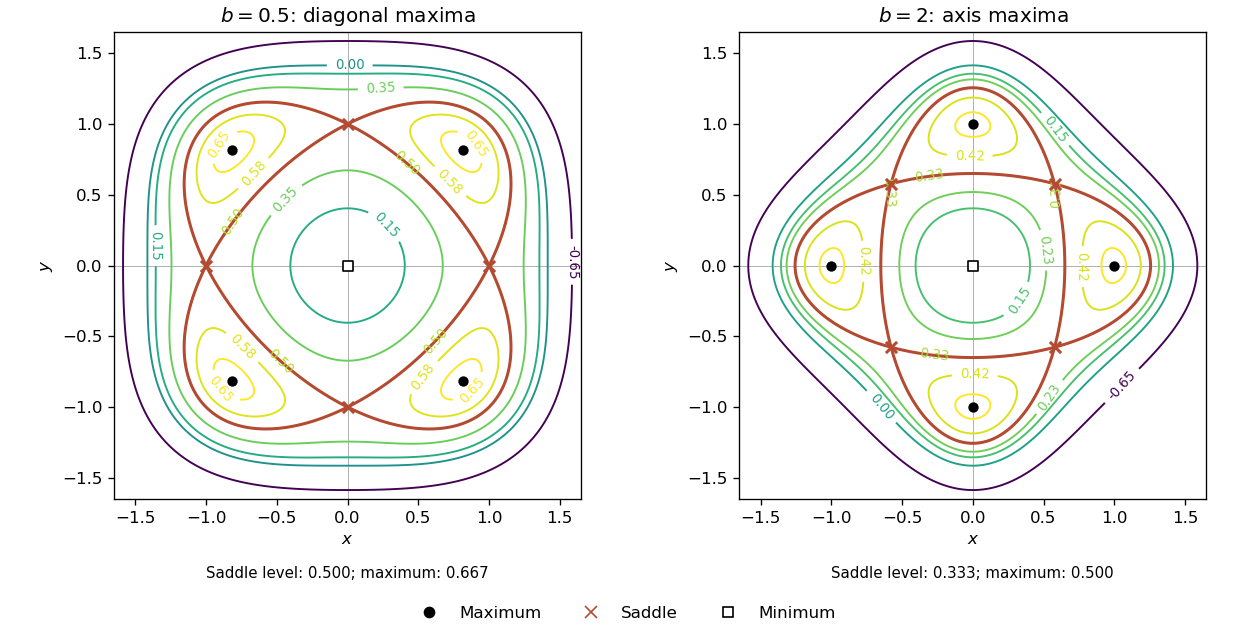
Contours of the fourfold quartic potential, with diagonal maxima for b less than one and axis maxima for b greater than one
. Details. 
Finally, at the expression depends only on radius:Consequently The maximum set is the whole unit circle, not merely four isolated points.
Let be the offspring probability generating function, and let , for . Given , the next generation is a sum of independent offspring counts. Multiplication of their probability generating functions givesTaking conditional expectation and then averaging provesThus is the -fold composition of with itself. Induction makes this precise: it is true for , and composing once more gives the next generation. In particular , since both are the same iterated function. This is the generating-function recursion for a Galton-Watson process.
Write , initially assuming it is finite. The law of total expectation givesStarting at one therefore yields , with the value at understood to be one even if . Equivalently, differentiating the composition at one gives the same recurrence. If the offspring expectation is infinite, every positive generation has infinite expectation: a positive chance of at least one parent remains at each finite generation, and conditional on any positive parent count the next expected count is infinite.
For a Poisson branching process, . Extinction is absorbing because an empty generation has no parents, so extinction by generation is precisely . Hence . Using the composition in the order givesFor example is the chance of no offspring in the first generation. The recurrence includes the degenerate case , where extinction occurs in the first generation with certainty.
Put and track the difference between the numbers of wins. It is a biased random walk with increments and , stopped on first reaching or .
To finish at on game five, there must be four wins for and one for , with the final game won by . The unique loss for can be in position one, two or three. If it were in position four or five, the first three games would already have stopped the contest. Each of the three allowed paths remains strictly inside the barriers until the last step and has probability . By interchanging players, there are also three paths ending at , each with probability . ThereforeFor a fair game this is . Counting all five-game sequences with final win difference three would overcount paths on which the contest ended earlier.
This is a gambler's ruin hitting problem. For , let be the probability of reaching before when the current difference is . Conditioning on the next independent game givesStopping occurs almost surely: conditional on being inside the barriers, three consecutive wins by either player force absorption within the next three games. This event has probability , so the chance of surviving such blocks is at most , which tends to zero.
If , the characteristic roots of the interior recurrence are and , so . Imposing the two boundary values yieldsIn particular,For the recurrence instead has affine solutions, and the boundary values give , hence . The deterministic cases give zero and one respectively. The formula covers all of them continuously:The stopping argument and the boundary recurrence show why the answer concerns the first barrier reached rather than the win difference after a predetermined number of games.
Write . The inverse change of variables is , whose Jacobian determinant has absolute value . Completing the square givesThe change of variables formula therefore transforms the joint probability density function toIt factors into two normalized standard normal distribution densities. Thus and are independent variables; factorization proves the requested independence, rather than simply zero covariance.
The standard Gaussian random vector has a rotation-invariant density. In polar coordinates, , , its density with the area factor is , so the angular coordinate is uniform on an interval of length .
Put , so andIn the right half-plane, choose . The additional condition then requires . This wedge has angle ; its boundary has probability zero. ConsequentlyAt this is , as required by independence. The limits as and are and zero, respectively. The angular calculation is also the geometric basis of the Gaussian sign-correlation identity.
Use the positive-support convention for the geometric distribution and put . Differentiating the convergent geometric series givesConsequentlySubtracting the square of the expectation from the second moment yields
For the die, this is the coupon collector problem. When scores are still missing, let count rolls up to and including the next newly observed score. Every fresh roll has success probability , so has a geometric distribution of parameter . These six successive waiting times are independent: conditional on the entire past at the start of a stage, its waiting-time distribution depends only on the number , not on the identities of the missing scores. Iterated conditioning therefore factors their joint distribution. The total number of rolls is .
Using linearity of expectation givesUsing variance additivity for independent random variables, or the coupon collector waiting-time variance formula just derived by this decomposition, givesHence the requested standard deviation isThe hint rounds the sum of squares from to ; using that rounded value gives , consistent at the precision of the hint. The exact computation preserves the slightly more precise value above.
Articles were limited to the first 100 out of 216 total.
Articles by others on the same topic
There are currently no matching articles.