Use the separation vector from the star to the comet, and let . The two-body problem separates into uniform centre of mass motion andTaking a cross product with proves conservation of angular momentum; taking the scalar product with proves conservation of energy. The relative constants areThe total relative angular momentum and energy are and , respectively. The conserved eccentricity vector is . Its scalar product with gives , with the true anomaly. The periapsis and apoapsis distances are therefore and . Their sum is twice the semi-major axis, soAt either apsis ; substituting an apsidal radius gives . Thus the specific orbital energy implies the vis-viva equationThese are exact relative-coordinate formulas for an elliptic orbit, . In the barycentric frame the comet's speed is times the relative speed; the printed identification with the comet's stellar orbital speed uses .
The transverse velocity is . Subtracting its square from the vis-viva equation, and putting , givesConsequentlyThe positive branch is outward motion and the negative branch is inward motion. The PDF's unsigned expression gives the radial speed, or the outward branch, rather than the signed radial velocity everywhere. For example, on the inward part of any noncircular elliptic orbit, .
The same result follows from , with the true anomaly. The radicand is nonnegative precisely on ; it vanishes at periapsis and apoapsis. For a circular Kepler orbit, , and .
Assume spherical fragments of the common mass density , and let count fragments per unit diameter. Mass normalization of a power-law size distribution givesTheir geometric cross-sections are , hence the cross-section of a power-law fragment population is exactlyFor , large fragments dominate the mass integral and small fragments dominate the geometric cross-section integral. Neglecting the subdominant endpoints givesThe two actual error parameters are and . They must both be small; the approximation is not uniform as approaches either endpoint. At or the corresponding integral is logarithmic, so the endpoint-dominated formula must be replaced by that integral.
The printed line-density statement is incorrect for a phase-mixed orbit. A steady line density on a Kepler orbit is inversely proportional to speed: for a cross-sectional-area current , the area per unit arc length is . Equivalently, phase mixing gives , uniform in mean anomaly, where is the orbital period.
For an optically thin population of blackbodies in radiative equilibrium, a fragment absorbs and reradiates the same luminosity. Thus the fractional luminosity of a phase-mixed eccentric wire isThe specific angular momentum gives , so the integral is . Since ,This derives the intended result after explicitly correcting the density to .
The error is consequential. If one instead imposes the literal density , its time weighting is . Using , and givesAt this is times the printed result. The inverse-radius averages can also be obtained directly with eccentric anomaly , and .
Let be the parent comet's diameter, with the same mass density as the fragments, so . The required geometric cross-section is , using the corrected phase-mixed orbit interpretation.
Substitute this and the spherical mass into the endpoint-dominated fragment formula. The parent-body size from a fragment cross-section becomesThe common mass density cancels. The comet's radius is . This expression treats both fragment cutoffs as specified independently and has the same endpoint-approximation restrictions as part (iii).
If a model instead ties the largest fragment to the parent through , with fixed , one must solve that dependence too:That extra assumption is not supplied by the PDF; setting without saying so would change the requested size relation.
On the corrected steady phase-mixed orbit, each fragment crosses a fixed orbital longitude once per orbital period. Hence the cross-sectional-area current through that point isFrom the fractional luminosity of a phase-mixed eccentric wire, . Therefore the area rate at the foreground crossing of the line of sight isOnly the foreground segment blocks the star; the far-side intersection does not add another occultation current. The orbital area current is constant because the line density varies as , even though the local orbital speed varies.
Use an edge-on orbit and an equatorial, effectively central chord. Near the foreground crossing the radial velocity is along the line of sight; the projected transverse speed is . In the small stellar-angular-radius limit, , the crossing time is .
The cross-sectional-area current therefore places an areain front of the stellar disk. For an optically thin wire and a uniformly bright stellar disk, transit dimming by an optically thin orbital wire givesThis is a linear occultation estimate, requiring negligible overlap and a fractional dimming much smaller than one. A finite impact parameter shortens the chord; limb darkening, finite wire thickness and variation of across a large stellar angular extent modify the coefficient. The estimate cannot be extrapolated to dimming greater than unity.
Treat as instantaneous osculating orbital elements of the fixed-central-parameter Kepler orbit. The perturbing work changes the specific orbital energy according toThe specific angular momentum and conic equation giveSubstituting proves the Gauss planetary equation for the semi-major axis:Here denotes true anomaly, not the fractional luminosity used in Question 1. The equation follows from work alone; a normal perturbing acceleration has no instantaneous contribution because the velocity lies in the orbital plane. For slowly averaged evolution, the perturbation must be weak over one orbital period.
A blackbody grain absorbs starlight of flux and reradiates isotropically in its own rest frame. Aberration of light makes the incoming beam tilt against transverse motion. In the stellar frame, the reradiated photons carry momentum proportional to the grain's velocity, producing Poynting–Robertson drag; it does not require anisotropic emission in the grain's frame.
Define the radiation-pressure coefficientFor a spherical grain of radius and mass density , , assuming unit radiation-pressure efficiency. To first order in , the first-order stellar radiation force on a blackbody grain isThe incoming absorbed photon momentum contains the relative-flux factor ; reradiation supplies the additional . Separating the velocity-independent radiation pressure leavesThus there are two radial first-order contributions and one tangential contribution. The approximation assumes , steady absorption/reradiation and constant grain properties; a non-blackbody requires its actual optical efficiencies.
Put . The Poynting–Robertson drag acceleration has and . Its work is strictly dissipative:For an unperturbed elliptic orbit, use , and . Averaging over its orbital period givesSince , and , the Poynting–Robertson decay of a circumstellar orbit isFor a circular Kepler orbit this becomes . This is a secular first-order average, not an exact instantaneous decay law. If static radiation pressure is appreciable, use a bound conservative orbit with central parameter , requiring , and define its orbital elements accordingly; repeating the work calculation cancels and leaves the same coefficient .
Let , and . A tightly bound circumplanetary orbit lies well inside the Hill sphere, so and its orbital period is short compared with the planet's year. Treat the stellar flux and stellar direction as constant during one dust orbit. With stellar-frame velocity , the velocity-dependent acceleration isThe terms independent of , including the leading static radiation pressure, do no net work on an unperturbed closed circular orbit. HenceFor a coplanar circular orbit, and the component along the stellar direction has mean square . Thus yields the Poynting–Robertson decay of a circumplanetary orbitThe coefficient three assumes coplanarity, which the PDF does not state. For orbital normal , the general circular covariance is , givingAn orbital plane normal to the stellar radial direction has coefficient two during that orbit, a counterexample to an orientation-independent coefficient three. Averaging also over the planet's circular stellar orbit, with fixed dust-plane orbital inclination to it, gives coefficient . The conservative forces must be weak enough for the assumed approximately circular, planet-bound orbit to persist; the small planet-to-star mass ratio alone does not ensure this for arbitrary grain .
Keep constant. A circular circumstellar orbit stays circular in the secular drag approximation, and integrates to . The inspiral time under Poynting–Robertson drag to the stellar surface isThe final expression treats the star as a point, or assumes .
For the coplanar circumplanetary orbit used in the preceding result, , so . The inspiral time of circumplanetary dust to the planet's surface, for , isThus the timescales have the same dependence on stellar flux and , but planetary arrival contains a logarithm of the initial planetocentric radius. It is not always shorter: for a point star, only if . A constant tilted-orbit average replaces three by its appropriate orientation coefficient. Sublimation or other removal can terminate the evolution before either idealized arrival time.
Radiative drag is only one of several loss mechanisms. Around a star, radiation-pressure blowout can eject small fragments; its threshold applies specifically to zero-kick release from a circular parent orbit. Stellar-wind drag and gas drag can drive planetary migration, while sublimation destroys grains approaching high-temperature regions. Collisional cascades destroy or fragment grains and can feed the unbound size range. Planetary scattering can cause ejection, collision with a planet, or a stellar impact; resonant trapping of dust can instead delay planetary migration.
For circumplanetary orbits, collisions with the planet or its satellites, disruption in collisions, and escape under stellar tidal forces are additional losses. Orbits near or outside the Hill sphere need not remain planet-bound. Radiation pressure on circumplanetary dust can excite planetocentric orbital eccentricity or unbind very small grains; it need not act only through slow Poynting–Robertson drag. For charged grains, the Lorentz force in stellar or planetary magnetic fields can alter or destabilize an orbit. Shadowing of circumplanetary dust changes the radiation-force average and can reduce the quoted decay rate. Which mechanism dominates depends on grain size and composition, environment, orbit orientation and the available collision or gas density.
Use conventional mean longitudes and take the positive integers in lowest terms. Rotational invariance requires the angular coefficients of a resonant argument to sum to zero. Since the inner planet has zero orbital eccentricity, the eccentricity-type term involving its undefined apsidal angle has zero amplitude. The surviving outer-eccentricity argument isIts leading disturbing function term is proportional to . Near the period commensurability, is small, so the resonant argument is slow and repeated perturbations can add coherently. Trapping produces resonant-argument libration, rather than circulation, with .
A near-integer period ratio alone does not prove mean-motion resonance: the diagnostic is bounded resonant-argument libration. At this eccentric resonant term vanishes and is undefined. If have a common factor, reduce the ratio first; the unreduced is not the actual lowest resonance order.
In the mean-conjunction approximation set . The resonant conjunction geometry is thenThere are phase directions spaced by . The integer determines their temporal order: at exact resonance the synodic period is , and the conjunction longitude advances by per conjunction. For coprime this visits all branches; resonant-argument libration broadens each direction by about its libration amplitude of a resonant argument divided by .
Mean conjunction and actual alignment are different for an eccentric orbit. If is the true common longitude, write and , with the mean anomaly. Because while the circular planet has , the exact geometric relation isThe displayed equally spaced directions use , hence are leading-small-eccentricity geometry. With appreciable , use Kepler's equation to locate true conjunctions; equating true and mean longitudes silently is not exact.
In the weak, non-crossing, leading-eccentricity model the exterior resonant coefficient has positive sign: write its disturbing function as , with for the orders considered. The physical feedback can be seen for first order. Before an outer conjunction near apoapsis, the faster inner planet pulls the outer one backwards; after passing it pulls forwards. On the outward side, the nearer, stronger earlier pull wins, reducing the outer semi-major axis and increasing its mean motion. Thus is driven upward. On the inward side, the later forward pull wins and drives downward. The paired impulses cancel at the symmetric centre.
For higher order, sum the feedback over all conjunction phases. The first surviving angular Fourier harmonic is ; the lower Fourier harmonics cancel over the equally spaced directions. A local Hamiltonian reduction with canonical momentum hasThe negative curvature of the Kepler orbit Hamiltonian gives the displayed sign. Linear stability analysis at gives a restoring acceleration. The symmetric libration centres of an eccentricity resonance are thereforeThe corresponding conjunction phases relative to periapsis are , and . They suppress repeatedly close passages and provide resonance protection.
These are expected centres of the specified leading-harmonic model, not centres fixed solely by the integer order for arbitrary orbital eccentricity and masses. Asymmetric resonant-argument libration can occur when higher Fourier harmonics matter. For example, if , , , the symmetric equilibrium loses stability and stable centres satisfy . Thus further dynamical information is needed beyond the PDF's unrestricted eccentric orbit to assert unique centres. Exterior asymmetric branches are documented by Winter and Murray, “Resonance and chaos. II. Exterior resonances and asymmetric libration”.
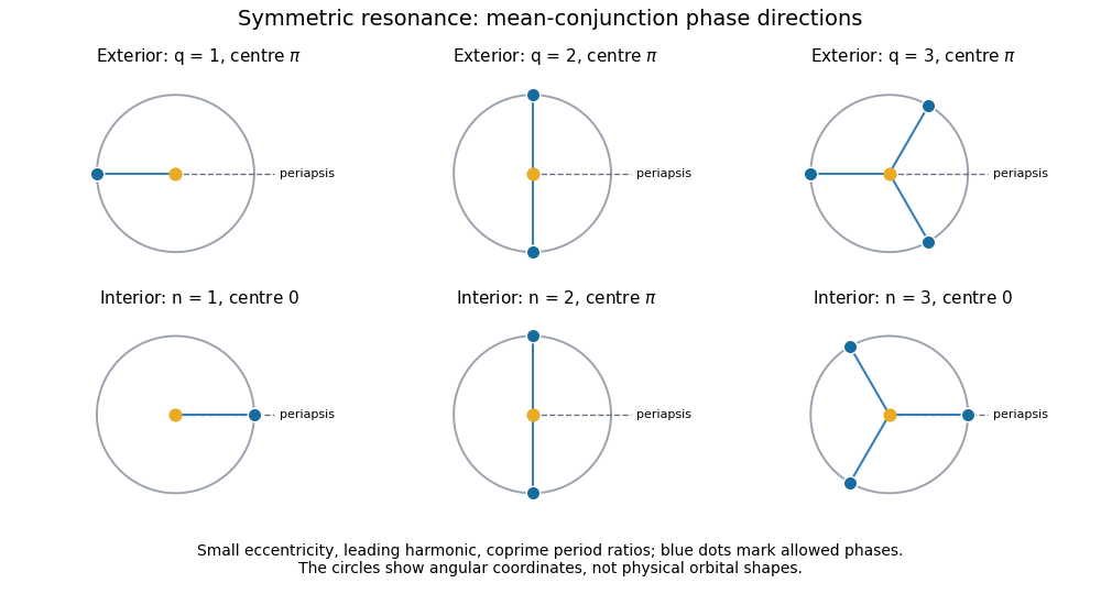
Mean-conjunction phase directions in symmetric orbital resonances
. Leading-eccentricity mean-conjunction phases relative to periapsis, with exterior and interior symmetric resonant-argument libration centres. Details.
Now the eccentric planet is inside the circular perturber . The interior eccentricity-type mean-motion resonance hasIn the mean-conjunction approximation, , so . Successive conjunctions advance by ; coprime visit distinct phases.
The near-conjunction tangential pulls are reversed for an eccentric body inside its perturber. Just before conjunction the inner body is pulled forwards and afterwards backwards. Near periapsis, an inward-moving inner body experiences the stronger earlier forward pull; its semi-major axis grows, its mean motion falls, and increases because its coefficient of is negative. On the outward side the feedback reverses, restoring the first-order centre zero. Higher-order feedback is strongest on the side closest to the external perturber, near apoapsis; the leading coefficient alternates in sign with order.
Writing gives for odd and for even in the leading non-crossing model. The same negative-curvature Hamiltonian argument therefore givesConjunction phases relative to periapsis are , and , respectively, as shown in the lower row of the figure. As before, these are small-eccentricity symmetric predictions; additional resonant Fourier harmonics and coupled secular dynamics can change the stable branches.
For actual alignment of the eccentric body at true longitude , the exact phase relation is instead , where and . The simple equally spaced angles replace by at leading order.
A simultaneous transit in a resonant chain requires both conjunction patterns to admit the observer's longitude at the same time. In the leading mean-conjunction geometry put . The necessary phase compatibility at symmetric centres isLet . Eliminating , and using that ranges over multiples of , gives the exact modular compatibility criterionHere denotes the greatest common divisor. For the orders above, the two phase sets intersect only whenThe common directions are the two quadratures relative to periapsis. In reduced resonances this requires and odd; otherwise the apparent second-order ratios reduce to different resonance orders. There is no additional restriction on those odd values from angular compatibility alone. A shared direction and suitable temporal phase can be chosen, and the rational period ratios allow its recurrence.
This is a potential low-amplitude configuration, not a guarantee of an observed triple exoplanet transit. The observer must lie in the common orbital plane and near an allowed direction. Finite stellar radii, nonzero libration amplitudes of a resonant argument, apsidal motion and asymmetric centres broaden or change the possibilities. At finite , true simultaneous alignment obeys the more precise equations and , with . Thus the order-only conclusion is not a universal necessary condition for every eccentric resonant chain.
First adopt the uniform-angular-motion approximation implicit in the requested formula. Set the line of sight to longitude zero, the exoplanet transit to , and the next exoplanet transit to , with . Write , , with . The next conjunction satisfiesThe common longitude is modulo . Subtracting one gives the conjunction longitude from a transit time lagSubstitution of the period ratio yieldsIt is exact in this uniform-angle model; no first-order expansion in is necessary here. For other choices of which exoplanet transit is used, choose the appropriate whole-turn branch.
For the finite-eccentricity orbit specified earlier, this is an approximation. Let and be the true anomaly and mean anomaly at the line of sight. The eccentric planet has and true angular advance , whereTrue conjunction therefore requires . The PDF omits this term, which is generally .
For a concrete counterexample take , , , , and a line of sight along 's periapsis. The uniform model predicts and longitude . At that time , but Kepler's equation gives , so the planets are not truly aligned. Accurate finite-eccentricity conjunctions must be found from the corrected equation.
For constant mean motions, consecutive mean conjunctions are separated by and advance in longitude by . To follow one of the branches, compare conjunctions steps apart. At exact resonance that advance is ; subtract it to measure the slow drift. Hence conjunction-pattern precession near a mean-motion resonance isThe printed expression is its leading small-offset term:Positive gives retrograde drift and negative prograde drift. The tracked-branch rotation time is about ; the full set of interchangeable directions repeats after a rotation , giving the usual mean-pattern super-period . The slow, continuously tracked branch interpretation assumes the resonance neighbourhood ; merely need not give a slow pattern for an arbitrarily large integer ratio . At there is no offset-driven drift.
The allowed directions can consequently move through the observer's line of sight. Triple exoplanet transits require the and patterns, together with their timing phases, to overlap that line of sight within the finite exoplanet transit windows; differing drift rates can open and close such windows. A small offset neither guarantees a triple event nor prohibits it permanently.
Moreover, in a true mean-motion resonance, bounded can coexist with a period offset because . The mean conjunction pattern then follows apsidal precession plus the resonant-argument libration correction. For appreciable orbital eccentricity, the true-conjunction geometry has the periodic corrections identified above; the drift calculation is a mean-phase result.
Let be the separation of the two centres at release. The two-body problem has relative specific orbital energy . Marginal escape has , soThis follows equally by equating the relative kinetic energy to the magnitude of the Newtonian gravitational potential energy , where .
For a pointlike comet released at the planet's surface, , giving the usual . If the finite comet touches that surface, its centre is at ; the same formula uses this larger separation. The assumption by itself does not imply . Subsequent formulas written in terms of the planet-only escape velocity use the additional small-comet approximation.
This is local escape from an isolated planet. In a stellar Newtonian gravitational field, reaching the edge of the Hill sphere and escaping the stellar system are different energy thresholds.
Work in the planet's rest frame, neglecting its recoil and tidal forces during the close encounter. A hyperbolic Kepler orbit has positive specific orbital energy and specific angular momentum , where is the impact parameter. Its orbital eccentricity isAt the pericentre distance, . Substituting yieldsThe two asymptotes have true anomalies , where . Their directions of motion give the gravitational scattering angle , so . ThereforeAs a useful independent form, , displaying gravitational focusing. Here to the stated small-comet accuracy; the exact relative-coordinate formula replaces it by .
The incoming and outgoing velocity vectors have the same magnitude , by conservation of energy. The chord between them has lengthFor fixed put . Then , and proves . Equality occurs at .
A non-colliding comet must have , where in the point-comet approximation and for finite bodies. Thus the non-colliding gravitational velocity-kick bound isThe optimizing grazing orbit has , and . If contact itself is excluded, this is a supremum approached from larger . The finite collision radius is essential: an ideal point planet with unrestricted has no finite upper bound.
A constant Galilean boost by the planet's stellar orbital velocity leaves the vector difference unchanged. It changes the comet's incoming and outgoing heliocentric energies, which is the basis of a gravitational assist.
Let , with . The Safronov number is . In the instantaneous planet frame let the asymptotic vectors be and ; their magnitudes agree. In the stellar frame the corresponding specific orbital energy change during a short encounter isThe quadratic relative-speed terms cancel. A comet with semi-major axis comparable to has stellar binding energy per unit mass of order . Consequently measures whether a single strong encounter can change a substantial fraction of that binding.
Large escape-to-orbital-speed ratios favour ejection; small ratios favour collision or accretion during repeated encounters. For , a suitably oriented gravitational assist can eject the comet before it strikes the planet. For , most individual kicks are too weak; many close passages may be needed, providing repeated chances of collision.
The crossover is of order unity, not a sharp theorem about each orbit. The initial binding energy, encounter speed and geometry matter: an already nearly parabolic comet may be ejected by a low- planet, while an unfavourably directed kick can make a comet more tightly bound even when is large.
For a spherical planet of mass density , . The point-comet surface escape velocity and circular Kepler orbit speed therefore giveRaise this equation to the power and solve for :Thus the constant of proportionality is , and the gravitational constant cancels. Dimensional checking gives mass on the right: has that dimension.
This uses the planet's own escape velocity. If instead is defined at finite-comet contact, an additional factor appears on the right, and itself depends on ; the quoted pure-planet scaling is then only the limit.
Write for the comet's inverse semi-major axis. Its specific orbital energy is , so escape corresponds to . The printed quantityhas dimensions of inverse length. It cannot, literally, be a standard variance-per-time diffusion coefficient. Interpret it as the characteristic root mean square step in per periapsis passage, as in a discrete comet energy diffusion model.
If successive kicks are unbiased and uncorrelated, after passages the root mean square displacement is . Starting at gives , hence . Taking the characteristic interval to be the initial orbital period givesHere . In particular, for this is . Without specifying the initial semi-major axis and the time per statistically independent encounter, the PDF cannot determine a unique time.
With the convention , the actual diffusion coefficient would be . The estimate requires , orbit crossing, and sufficient phase decorrelation. Near escape the orbital period grows, and resonant or secular correlations invalidate the simple constant-step clock. This is a characteristic diffusion scale, not an exact mean first-passage time: even an unbiased Brownian motion on an unbounded half-line has an infinite mean time to reach its absorbing endpoint.
Fix and an initial-orbit ratio ; use for the figure. The qualitative finite-age planetary scattering regimes have two useful boundaries.
First, the order-unity escape-to-orbital-speed boundary isIt slopes down with logarithmic slope . Above it a planet can give large fractional binding-energy changes, favouring planetary ejection of a comet; below it weak kicks and repeated collision opportunities favour accretion.
Second, equating the characteristic comet energy diffusion time to the age givesThis boundary slopes up with logarithmic slope . Above it the many-encounter diffusion estimate fits within the available age; below it that estimate exceeds the age.
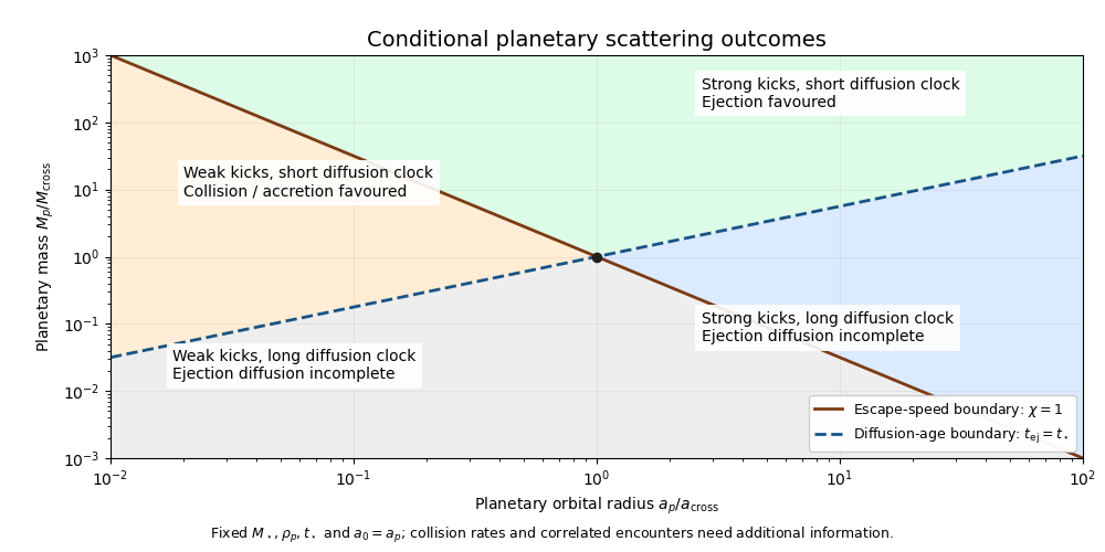
Regimes of planetary scattering and ejection
. Qualitative planetary scattering map at fixed stellar mass, planetary mass density, age and . The axes are normalized to the intersection of the and boundaries. Details.
Above both boundaries, rapid ejection is favoured. Above the age boundary but below the escape-speed boundary, repeated encounters can act during the age while individual kicks remain weak, so collision or accretion is commonly favoured. Below the age boundary, the diffusion model predicts incomplete ejection; the escape-speed boundary still distinguishes strong from weak individual kicks.
These labels are statistical expectations under the stated encounter model. In particular, the given diffusion coefficient supplies no collision rate, so it does not prove that every object in the low- region is accreted within . Nor does a long ejection time exclude faster collisions or other loss mechanisms. Very massive planets with require a few-encounter treatment rather than an extrapolation of the diffusion formula.
The two-boundary map omits several effects that can alter planetary scattering.
The initial semi-major axis, orbital eccentricity, orbital inclination and orbital phase determine whether encounters occur and their relative velocities. A strongly bound comet needs more energy to escape; a nearly parabolic one needs less. The planetary radius and mass density, the finite comet radius, and gravitational focusing determine collision probabilities. Tidal disruption, atmospheric gas drag, sublimation and physical fragmentation can destroy a body before a nominal point-particle scattering sequence is completed.
Other planets can hand a comet from one scatterer to another, eject it, or lift its periapsis clear of the original scatterer's orbit. Mean-motion resonances and secular perturbations can protect objects from encounters or correlate kicks, contradicting the independent random walk assumption. Planetary migration changes the encounter geometry over time.
Stellar flybys and a galactic tide can change distant comet periapses, allowing new encounters or detaching an object from the planetary region. Stellar mass evolution changes both binding and planetary orbits. Finally, the age and the supply rate of new comets determine whether the observed population is a residual one or continuously replenished. Thus the mass-radius map is a useful conditional classification, not a complete survival law.
Articles by others on the same topic
There are currently no matching articles.