Solutions to all six questions of the examination sat on 23 June 2023, including every optional question and part.
Let be a bounded planar region with a piecewise smooth, simple closed boundary , oriented counterclockwise, and let have continuous first partial derivatives on an open neighbourhood of its closure. Green's theorem states thatFor a region with holes, orient every boundary component with on its left: the outer component is counterclockwise and the inner components are clockwise.
Choose and . Their indicated partial derivatives differ by one, so the area isThis is signed area as a boundary integral; reversing the direction of changes the sign of the integral.
In polar coordinates, put and . Differentiating along the curve givesThe cardioid has and is traversed once counterclockwise as increases from to . Its cusp at causes no difficulty: split the line integral there, or exclude a small arc and take its limit. Thus signed area as a boundary integral gives
For an oriented piecewise smooth parametric curve and a continuous vector field along it, the vector-field line integral isFor a piecewise smooth curve, sum these integrals over its smooth pieces. The dot product selects the component of the vector field in the direction of motion.
If for a smooth function , the multivariable chain rule givesThe fundamental theorem of calculus, with cancellation at intermediate endpoints, therefore proves the fundamental theorem for line integrals:On a closed curve , so .
The displayed vector field is defined on the punctured plane ; it is undefined at the origin. Take the counterclockwise unit circle , . Along it,By the fundamental theorem for line integrals, it has no single-valued potential of a conservative vector field on . In particular it cannot be the restriction of the gradient of a smooth function on all of .
For , direct differentiation givesThere is no contradiction with Green's theorem: is not defined, let alone continuously differentiable, throughout the disk enclosed by . On an annulus the theorem does apply; the counterclockwise outer integral is , and the clockwise inner integral is , so their sum is zero. The hole prevents this curl-free vector field from being a conservative vector field on its entire domain.
For a continuous vector field along an oriented piecewise continuously differentiable parametric curve , define its line integral byadding the integrals over the smooth pieces when necessary. The value refers to the specified traversal: going around a curve twice counts twice.
An orientation-preserving reparametrization has the form , where is an increasing, piecewise smooth change of parameter with , . For regular parametrizations one may take and its inverse continuously differentiable on each piece. The chain rule gives . The change of variables therefore yieldsThis proves reparametrization invariance of a vector line integral. If is decreasing, the endpoints in the final integral are reversed and the sign changes. Thus the same direction and the same multiplicity of traversal are essential.
For the parametric curve , , the vector field and the tangent vector areConsequently the line integral is
Compute the line integral on each straight segment. On the first, and only contributes; on the second, and only contributes; on the third, and only contributes. ThereforeAlthough on the second segment, that term does no work there because .
Parametrize the straight segment by , . Then the line integral isThe three different answers are possible because this vector field is not a conservative vector field; for example whereas .
Take counterclockwise traversal as viewed from . In the plane , the work is the planar line integral of and . Green's theorem givesThe component contributes nothing because . The question specifies one circuit without specifying its direction: clockwise traversal gives .
Let be a piecewise smooth oriented surface, and let be continuously differentiable on an open neighbourhood of it. Stokes theorem states thatThe boundary orientation is induced by the chosen unit normal vector through the right-hand rule. Smoothness on a neighbourhood makes the spatial partial derivatives in the curl well defined.
Choose the outward orientation of a surface on the lower half of the ellipsoid. At its lowest point the normal points down, so its boundary ellipse is traversed clockwise when viewed from above. UseThe line integral is
For an independent surface integral calculation, first compute . Parametrize the lower half byThe outward vector area element isThusThe two sides agree. Choosing the inward unit normal vector and its corresponding counterclockwise boundary orientation changes both answers to .
The sufficiency claim requires a domain qualification. For a continuously differentiable vector field on all of , or more generally on a simply connected open domain, the equivalence is valid. On an arbitrary domain, vanishing curl is necessary but may fail to be sufficient.
Necessity. Suppose every closed-curve line integral vanishes. Fix a point in the open domain and a unit vector . A sufficiently small planar disk of radius , centred at and normal to , lies in the domain. Stokes theorem givesDivide by and let . By continuity, the average tends to . Taking the three coordinate directions proves everywhere.
Sufficiency on . A direct proof constructs a potential of a conservative vector field. PutWrite for the components of . Vanishing curl says . Differentiation under the integral, followed by the chain rule, givesThis is the radial integral potential for a curl-free field. The fundamental theorem for line integrals now gives zero on every closed curve. On a simply connected open domain the analogous argument uses path integrals: every loop can be contracted within the domain, and applying Stokes theorem to a piecewise smooth contraction makes its circulation zero. Equivalently, whenever a particular loop bounds an oriented spanning surface entirely in the domain, Stokes theorem immediately gives zero for that loop.
Why the domain matters. On , the smooth vector fieldhas zero curl, but its line integral around the unit circle in is , as in ii. No spanning surface for this loop can lie entirely in . The literal claim without a condition on the domain therefore has this counterexample.
Let be an arbitrary constant vector. By the cyclic identity for the scalar triple product,Apply Stokes theorem to . Since is constant, the curl product identity givesConsequentlyFor precision, the operator in the last line has componentsThe partial derivatives act on , with multiplying their values; they do not differentiate . Since the dot products agree for every constant , the cross-product form of Stokes theorem follows:Here in the paper denotes the cross product, and the printed surface integral has its area element understood.
For the Fourier cosine series, first take the even extension on , and then its -periodic extension. Evenness eliminates the sine terms. With the constant term written as , the Fourier coefficients and series areFor the Fourier sine series, take the odd extension for and for , and extend with period . Values assigned at isolated endpoints do not change the Fourier coefficients. Oddness eliminates the constant and cosine terms, leavingBoth formulas follow by orthogonality on and the parity of the extensions.
Using the usual piecewise smooth interpretation of the derivative hypothesis, Dirichlet's theorem on Fourier series gives the average of the two one-sided limits of the appropriate periodic extension. The even extension is continuous at and at the identified endpoints , so the Fourier cosine series converges toFor the odd extension, the one-sided limits at zero are and , while at the periodic one-sided limits are and . Hence the Fourier sine series converges toAt an endpoint this equals precisely when is zero there. One can also see the zero endpoint values directly: every partial sum consists of sines that vanish at both endpoints.
Put . The constant Fourier coefficient isFor , integration by parts givesThe terms cancel. ThusThis Fourier cosine series has when is divisible by four, when , and when is odd.
The Fourier cosine series converges to the continuous even -periodic extension. If represents modulo , its value isIt has value zero at , rises linearly with distance from these points until height , and then stays flat until the next descending ramp. Thus the sketch on has minima at , and plateaux centred at the odd multiples of . Its large partial sums round the corners and closely follow the whole graph.
The Fourier sine series converges, away from the odd multiples of , to the odd -periodic extensionAt every odd multiple of its value is zero, the midpoint of the jump from to . At even multiples of it passes continuously through zero. Thus on every interval it has a negative plateau, a rising linear segment through , and a positive plateau. The jump size is .
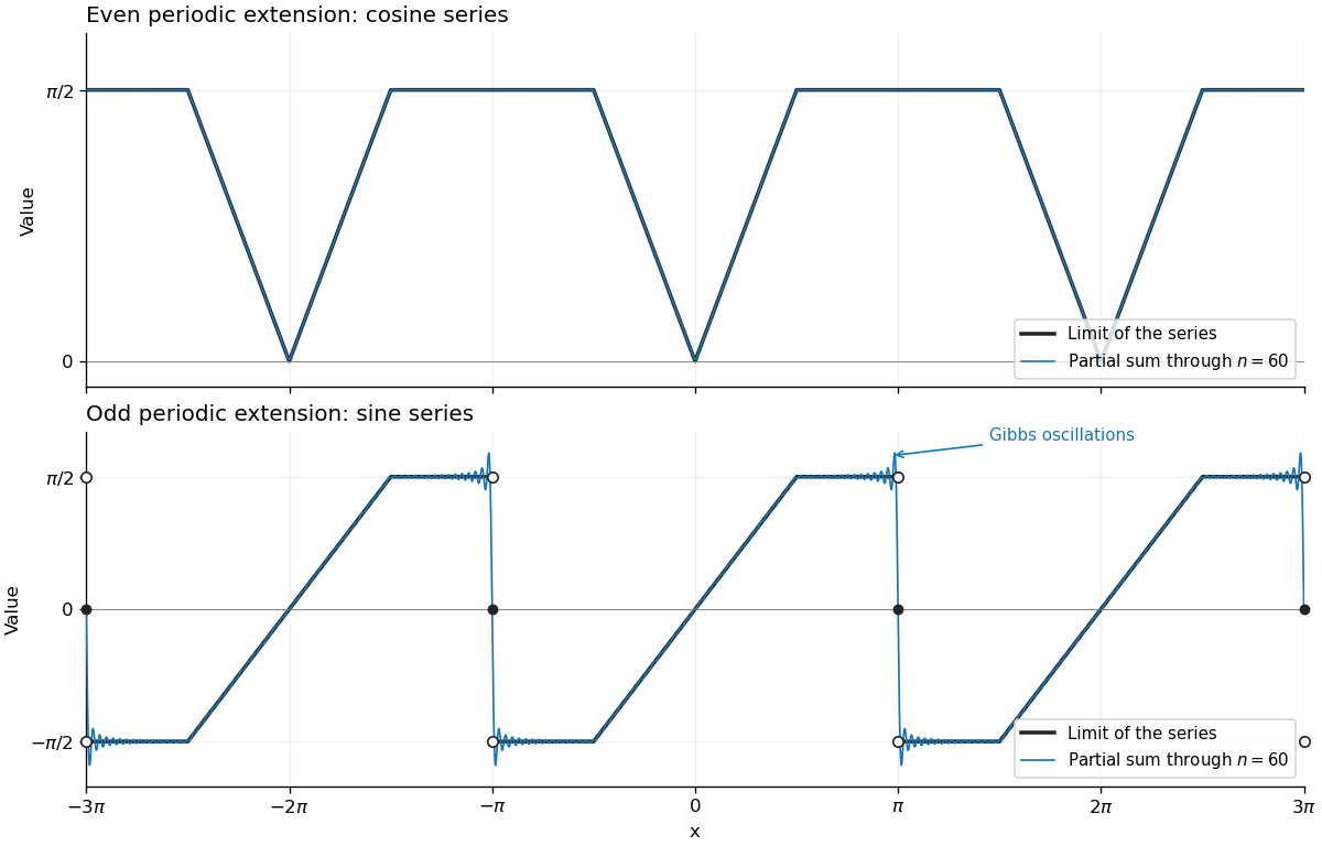
Periodic limits and 60-term Fourier partial sums
. Details. The blue curves are the partial sums through . The open endpoint circles and filled zero dots in the lower panel distinguish the one-sided limits from the value of the Fourier sine series at each jump. Near these jumps the partial sums exhibit the Gibbs phenomenon: the oscillations become concentrated in narrower regions as the number of terms grows, while their limiting overshoot remains about times the jump, here about .
The truncated Fourier cosine series gives the better approximation over the whole closed interval. Its Fourier coefficients obey , so absolute convergence and the tail boundgive uniform convergence. The even periodic extension is continuous; its slope changes only cause corners.
By contrast . The odd periodic extension has a jump at , giving slower coefficient decay and the Gibbs phenomenon near that endpoint. Every truncated Fourier sine series satisfies , soIt therefore cannot converge uniformly to on , although it converges at every point of . This comparison concerns approximation across the interval; it does not assert that the cosine truncation has smaller error at every individual interior point for every .
Take a bar of constant cross-sectional area , thermally insulated along its sides, with no internal heat production. Fourier's law says that the heat flux in the positive direction isThe thermal conductivity is positive. On a small slice , conservation of energy givesHere is the volumetric heat capacity, the product of mass density and specific heat capacity. Divide by , take , and use . The resulting heat equation isFor differentiable , this is ; retaining the divergence form also expresses conservation of energy correctly across an interface where jumps.
Inward heat flux at the left end points in the positive direction, so the boundary conditions areFor uniform thermal conductivity, the steady heat equation gives . The heat flux is constant and equal to , so . Imposing the right-end temperature gives
Write . The transient satisfies the heat equation and homogeneous mixed boundary conditionsThe left condition is a Neumann boundary condition and the right one a Dirichlet boundary condition. Separation of variables, , givesThe condition removes the sine term. The condition then selectsThere is no nonzero mode with , because a linear satisfying both conditions is zero. There is no growing mode either: integration by parts gives , so every nonzero mode has .
These Sturm-Liouville eigenfunctions have orthogonality and squared normExpand the initial transient in this half-integer Fourier cosine series. Its coefficients areThe integration formula follows by integration by parts; the cosine at the endpoint is zero. Thus the half-integer cosine expansion of a linear profile givesAt the Fourier series reproduces everywhere, including the endpoints; its coefficient decay gives uniform convergence. For every the exponential factors allow termwise differentiation and verify the heat equation and both boundary conditions. The sudden switch-on of nonzero heat flux is incompatible with the spatial derivative of the constant initial temperature at the corner . Accordingly, the positive-time boundary derivative must not be inferred by differentiating the initial Fourier series term by term at that corner.
For the stated inward heating, take and put . Since , the transient from ii satisfiesEquality holds at , where every cosine is one and all coefficients have the same sign. Thus the maximum is attained at the heated end, and its exact value and late-time form areThis is dominance of the slowest-decaying eigenfunction when . More explicitly, the omitted relative correction is nonnegative and bounded by , using . For a signed imposed heat flux, the maximum-deviation formula uses .
In a steady state the heat equation says , so the positive- heat flux is the same constant in both materials. Assume perfect thermal contact: temperature is continuous at , and conservation of energy requires continuous heat flux there. Integrating from the right endpoint givesThe two formulas agree at the interface. Their slopes differ, but . The total temperature drop is , the sum of the two layers' contributions in steady heat conduction through layers.
Use the ideal transverse-motion model of the question: constant tension, small slopes, no bending stiffness, and no transverse body-force term. On a short segment away from , the vertical components of the endpoint tensions are, to first order in , and . Its mass is , since is linear mass density. Newton's second law givesDividing by and taking its limit proves the wave equation on a string on each side of the mass:The string on the right pulls the point mass with vertical component , while the string on the left contributes . HenceThe fixed supports and attachment impose the boundary conditionsTogether with the mass equation, these are the endpoint and matching conditions. The slope can jump at : the jump supplies the mass's vertical acceleration. Requiring the slope to be continuous would incorrectly remove its dynamics.
Use separation of variables to seek a normal mode , with angular frequency and wavenumber . The endpoint boundary conditions are built intoLet and denote the mass's displacement amplitude by . Continuity and the mass equation becomeThe two possibilities must be separated before dividing by .
Antisymmetric modes. If , then , , and . The force equation gives , since . Thus and the mass stays at rest. These allowed angular frequencies satisfyThe restoring forces on the mass cancel even though the string vibrates.
Symmetric modes. If , continuity forces . Cancelling the nonzero amplitude in the mass equation and using givesThese modes have and move the mass. In dimensionless form their equation is , where . This is the spectral splitting for a string with a central point mass.
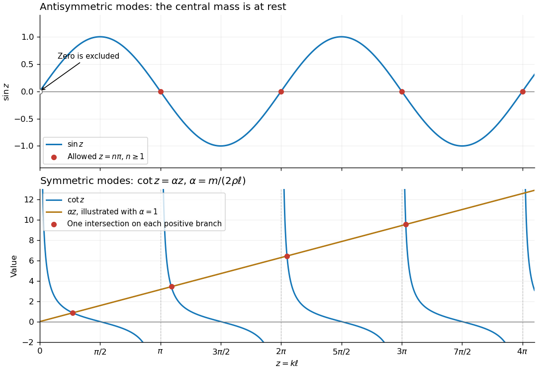


For the antisymmetric family, the graph of crosses zero at every positive multiple of . For the symmetric family, on each interval , , the graph of decreases continuously from to zero while increases. By the intermediate value theorem and strict monotonicity, there is exactly one intersection in each interval. On the remaining half-intervals , so there are no further positive roots. This proves graphically and analytically that both families contain infinitely many normal modes. The figure uses for illustration.
The algebraic case is not a mode: a zero-frequency profile would be linear on each half, continuous and zero at the endpoints; the zero-acceleration mass equation also makes its slopes agree, forcing the entire profile to be zero. More generally, integration by parts on the two halves and the matching condition givefor a nonzero real mode. Thus no nonzero static or exponentially growing mode has been omitted.
The lowest positive root belongs to the symmetric family and lies in ; all antisymmetric roots are at least . Let . The equation forces its first root to tend to zero: for any fixed , the right side eventually exceeds at , so the decreasing-minus-increasing difference has its zero below .
The Taylor series then givesSince and , the lowest angular frequency isPhysically, at such a low frequency each half-string is nearly straight. If the mass moves up by , the two slopes are approximately and , so the restoring force is . The resulting harmonic oscillator equation, , has exactly the leading angular frequency above. The next correction from the same expansion is .
Articles by others on the same topic
There are currently no matching articles.