These solutions cover all ten questions, including every printed subpart. The original PDF supplies the adjoints in Question 5, the fourth powers in Question 7 and the complete Question 10. Two qualifications to the printed wording are explained where they arise: unitary diagonalisation in Question 5 and the integration limits in Question 10.
Coordinate surfaces and sketch. Adding and subtracting the defining relations gives and . Since , we have . For , eliminate to obtainThis is a parabolic cylinder parallel to the axis, opening towards negative , with cross-sectional vertex and focus at the origin. Similarly, givesa parabolic cylinder opening towards positive , with vertex and the same focus. The degenerate surface is the half-plane ; gives . Constant gives the horizontal planes .
Thus the requested cross-sections consist of , , , and the two horizontal half-axes. The parabolas of the two families meet orthogonally.
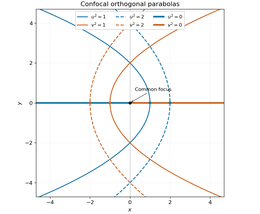

Signed coordinates. Take and choose the sign of to agree with away from . Then the Cartesian coordinates areEvery coordinate triple gives exactly one point. For , and have the same sign. A fixed signed selects the upper or lower half of its parabolic cylinder; the entire cylinder corresponds to fixed . On the cut , the two values represent the same point of the negative half-axis. This boundary identification is unavoidable: there even when , so the sign prescription is understood by approaching from either side of the cut. The interior gives a unique coordinate chart off that half-axis.
Orthogonality and metric. Differentiate the position vector:The pairwise dot products vanish. Their lengths give the scale factors of orthogonal coordinates and hence the Riemannian metric:These are parabolic cylindrical coordinates. The differential calculation is regular for ; the axis is the coordinate singularity where the two planar tangent vectors vanish.
Laplacian. Put . The physical components of the gradient of a -independent scalar field are . Applying the divergence formula cancels the two equal scale factors of orthogonal coordinates inside the derivatives:Therefore, away from the coordinate singularity,
Steady state. In the heat equation, time independence makes the second spatial derivative zero. The two endpoint temperatures therefore determine the linear profileInsulation is along the sides; the endpoint reservoirs can still exchange heat with the rod.
Transient solution. Subtract the steady profile before applying separation of variables: let . Then , and for . Writing givesThe homogeneous Dirichlet boundary conditions exclude and select the eigenfunctions with eigenvalues , . Their orthogonality gives the Fourier sine series coefficientsHere integration by parts uses . ThusEvery summand satisfies the heat equation and the homogeneous endpoint conditions, while the steady profile supplies the prescribed endpoint values. The initial Fourier sine series equals in the open interval. At the initially cold rod and the suddenly imposed hot endpoint are incompatible; the formula describes the prescribed data for and the initial limit at interior points.
Heat absorption. Integrating in kills the even modes. With , the total heat relative to the initial state isConsequently the net rate of heat absorption isFor each , any fixed number of differentiated modes is bounded by a polynomial in times . These bounds have finite sums, proving absolute convergence, uniform convergence on such time intervals and the validity of the integration and differentiation. In particular the displayed rate is finite for every , positive when , and tends to zero as equilibrium is approached. The same answer follows from the heat equation balance ; this subtracts loss at the cold endpoint from input at the hot endpoint.
Transform convention and derivatives. Use the Fourier transform pairFor sufficiently decaying with integrable second derivative, two applications of integration by parts giveThe identity also holds for tempered distributions, which is the setting needed for the Dirac delta function boundary data.
Upper half-plane solution. Take the Fourier transform in only, writing . Laplace's equation becomes . For , discard the exponentially growing solution and use , the Fourier transform of the Dirac delta function. This gives . The value at can be set to its continuous limit one. Pointwise decay of as does not require this individual transformed value to decay: the total integral in remains one while the profile spreads.
The inverse Fourier transform now yields, for ,Evaluate the last integral as the real part of :This is the Poisson kernel for the upper half-plane. Its boundary condition is a distributional convergence, rather than an ordinary value at : for a smooth compactly supported test function ,The dominated convergence theorem applies because is bounded and is integrable. Also , proving the required decay as .
Direct verification. Differentiating the rational expression givesTheir sum is zero throughout , so the solution is a harmonic function there.
Nilpotence and eigenvalues. If with , then . Thus forces for every eigenvalue. Conversely, if all complex eigenvalues, counted with algebraic multiplicity, vanish, the monic characteristic polynomial is . The Cayley-Hamilton theorem then gives . HenceThis is the criterion for a nilpotent matrix.
Symmetric case. Here a symmetric matrix is understood to be real. The spectral theorem gives with orthogonal and real diagonal. The previous result makes every diagonal entry zero, so . Alternatively, choose , so . For every real vector ,It follows that . Repeat until . This uses positivity of the quadratic form . The restriction to real symmetric, or complex Hermitian matrices, matters: a complex matrix satisfying only need not have this positivity.
The parameters and powers. The first two columns of coincide, so for all . The sum of its principal two-by-two determinants, each a minor of a matrix, isTogether with , this givesFor every eigenvalue to vanish both remaining coefficients must be zero. ThereforeDirect multiplication at these values givesIndeed the first row of multiplied by is , and the second row is its negative.
Geometry of repeated application. For any parameters the image of a linear map lies in the span of and , since . Thus it lies in a fixed plane through the origin, independently of the input. When are independent its normal is ; if they coincide, the image is a line and is still contained in a plane.
For , put and . ThenThe columns span this entire plane, so has rank two. The next two steps areThus the image of a linear map contracts from a plane to a line and then to the origin under successive applications. The line from is precisely the kernel of .
The conjugate transpose reverses products and conjugates scalars. Since are Hermitian matrices,Therefore In particular the commutator of two Hermitian matrices is anti-Hermitian, and multiplication by converts it to a Hermitian matrix.
Suppose and . ThenBecause the eigenvalues of are distinct, the eigenspace for is one-dimensional. It follows that , including the possibility . Thus an orthonormal eigenbasis of is also an eigenbasis of . The simplicity of both spectra means their eigenvectors coincide as directions, up to ordering, phases and nonzero scalar multiples.
Conversely, if they share a complete eigenbasis, choose the unitary matrix whose columns are these common normalized eigenvectors. Then and are diagonal, so and . HenceThis is simultaneous diagonalization of the two Hermitian matrices.
The original PDF uses the conjugate transpose , rather than the transpose found in the transcription. The printed diagonalisation criterion is correct when diagonalisation means unitary diagonalization of a normal matrix. Since ,Consequently if and only if . By part (ii), this gives a common unitary matrix andwhich is diagonal. Conversely, if for a diagonal and a unitary matrix , thenThus the precise conclusion isIf arbitrary invertible changes of basis are allowed, the printed assertion is false. For example,satisfy . Both Hermitian matrices have distinct eigenvalues: for and for . The distinct eigenvalues make diagonalizable by similarity, but and differ. This distinguishes ordinary diagonalization from the required unitary version.
As is a unitary matrix, . Let . Its conjugate transpose is , so and every positive integer power are Hermitian matrices and have real eigenvalues.
More explicitly, if with real, then form an eigenbasis andThereforewhere denotes the matrix size, to distinguish it from the power .
Divide the Chebyshev differential equation by . Its coefficients and are analytic at zero, so The finite singular points of a differential equation are .
Insert , . The coefficient of the lowest power is , hence or . The next power gives , and the remaining powers yieldFor , is free andChoosing selects the even power series, with . For , the next-power equation forces andThis selects the odd power series, with . Their different initial values prove linear independence. Although the Frobenius method produces two possible leading exponents, zero is an ordinary point, and a general series already includes both initial constants.
Let for integer . In the even or odd power series whose parity matches , the numerator in the recurrence relation vanishes at the coefficient of . All coefficients of lower powers in that parity are nonzero, and all higher ones vanish. Therefore a polynomial solution exists, of polynomial degree , containingFor nonnegative these are the Chebyshev polynomials . The normalized low-degree cases follow directly from the recurrence relation:Enforcing givesTo see that normalization at one is always possible, set in the Chebyshev differential equation. For , the differential expression becomes . Thus gives on and has value one at . It is a polynomial because the cosine addition formula gives . Negative integer produces the same solution as .
Write a nonterminating parity series as , where or . Its recurrence relation isThe ratio test applied to its nonzero successive terms has limiting absolute ratio . Hence the series converges absolutely for and diverges for , withAt , the limiting ratio is one, so the basic ratio test alone is inconclusive. Retain the next term of the ratio instead:For large the ratio is positive. Taking logarithms and summing gives ; the remainders have a finite sum. Thus eventually. Comparison with the convergent p-series proves absolute convergence at both endpoints as well:The radius of convergence one is the distance from the expansion point to the nearest singular points of a differential equation, . Convergence of function values at those points does not make the solutions analytic there; endpoint derivatives can diverge. The terminating Chebyshev polynomial is an exception with infinite radius of convergence. For example, at the other solution is , whose endpoint values are finite while its first derivative diverges.
Multiply the differential equation by and compare the coefficients of and with . The required integrating factor satisfies . Thus one may takeThen , the desired Sturm-Liouville form, with the same homogeneous Dirichlet boundary conditions. A common positive constant multiplying is immaterial. For the usual regular Sturm-Liouville problem one also assumes real sufficiently regular coefficients and , ensuring .
Mixed endpoint spectrum. For , integration against and integration by parts, using , gives for every nonzero real eigenfunction. Thus and the first condition makes . The second requires , so , . Sincethe normalized eigenfunctions and eigenvalues areThe orthogonality also follows by applying integration by parts to two different eigenfunctions of the same self-adjoint differential operator.
Forced expansion. Let and write , . The Fourier coefficients of the forcing arebecause the boundary cosine vanishes and . Applying to the eigenfunction expansion gives . Since is not an eigenvalue,The coefficients are , so the series and its first two differentiated series converge absolutely and uniformly on the interval. Each term satisfies the two endpoint conditions, and equals the mixed-endpoint Fourier series of . The forcing coefficients are , giving uniform convergence of that series as well. Uniqueness follows because the homogeneous problem has a nonzero solution only at one of the excluded eigenvalues.
Odd fourth-power sum. Set . Direct integration of , with the same endpoint conditions, givesAt , the eigenfunction expansion instead gives . Equating the two values yieldsAbsolute and uniform convergence justify evaluation at the endpoint.
Use reduction of order by setting . Then and , so the differential expression simplifies toIn the homogeneous case is constant. Hence , and a basis of the solution space isTheir Wronskian is on , proving linear independence. No nonzero homogeneous solution satisfies both endpoint conditions: sets , and then sets .
Choose the homogeneous solutions , which vanishes at , and , which vanishes at . Their Wronskian in the order is . For a source point , seek the Green's function asIt is continuous at ; otherwise its second distributional derivative would contain a derivative of the Dirac delta function, which the source does not contain. Integrating the differential equation across the source, using continuity and the leading coefficient one, gives the jump conditionContinuity and this derivative jump requireSolving with the Wronskian gives and . ThereforeThe two values at are identical. The derivative jump is explicitlyBoth endpoint values vanish and the differential expression is zero off the diagonal, completing the verification of the Green's function.
By superposition, . Split the integral at : the portion uses the first branch of the Green's function, and the portion uses the second. This yieldsFor , put . The two integrals areSubstitution and cancellation giveIndeed . For a direct differential check,and thereforeThe homogeneous uniqueness shown in part (a) makes this the unique solution.
For the real Sturm-Liouville operator , two integrations by parts give the Lagrange identity for a Sturm-Liouville operator:Set . Both vanish at the endpoints, so the boundary term is zero. Since ,ConsequentlyThis is self-adjointness with the homogeneous Dirichlet boundary conditions, and expresses the Fredholm solvability condition at the eigenvalue . In this unweighted integral already contains its factor of ; adding another weight would be incorrect.
Assume the regular real Sturm-Liouville problem, with , ordered eigenvalues , and real orthonormal eigenfunctions in the weighted inner productThe Rayleigh quotient for an admissible trial function isThe second expression follows by integration by parts. It is the quantity used in the Rayleigh-Ritz method.
For , orthonormality eliminates every cross-term in the denominator:Applying to the eigenfunction expansion and using the same orthogonality in the numerator givesHence, whenever the trial function has finite energy,Put and . The exact error and its expansion areIn particular, under a common small scaling with fixed finite sums and ,The fourth-order remainder includes mixed products , not just individual fourth powers.
Error comparison and sign. Since , the relative weighted norm error of the supplied trial function isFor , the relative eigenvalue error is . Thus the Rayleigh quotient has a second-order error for a first-order error in the trial eigenfunction, provided the energy-weighted coefficient sum is controlled. Small weighted norm error alone does not control arbitrarily high-frequency contamination, because can grow without bound. If , an absolute error must replace the undefined relative one.
Finally every summand of is nonnegative. Thuswith strict inequality whenever some . This is the upper-bound property of the Rayleigh-Ritz variational principle for the lowest eigenvalue.
Let be a stationary function and perturb it to , where is smooth and . These perturbations preserve the prescribed endpoint values. Differentiate the functional at :By integration by parts,The boundary term vanishes. The remaining integral must vanish for every such , so the fundamental lemma of the calculus of variations gives the Euler-Lagrange equationIt is a necessary stationarity condition; deciding whether the stationary path is a minimum requires additional information.
Length functional. On the unit sphere, write the position vector in spherical coordinates asIts two coordinate tangent vectors satisfy , and . Consequently the induced Riemannian metric is . On a segment for which increases and ,Segments where is not monotone require another parameter or a subdivision. Endpoint turning points can be handled by a limit.
First integral. With , there is no explicit dependence. The Euler-Lagrange equation therefore says thatis constant. For , put and solve:The radicand must be nonnegative along the chosen segment. The printed expression with both limits fixed at describes a longitude difference between endpoints; a formula for needs the variable upper limit and the additive constant shown here. The case gives a meridian with constant longitude. The equator is also a stationary route, although it cannot be parameterized using changing .
Integration and geometric meaning. Put , so andFor a nonconstant segment , and writing , the integral becomesRearranging, and absorbing phase and sign into two constants, givesMultiplying by shows that the corresponding Cartesian coordinates satisfy . Thus every such stationary route lies in a plane through the sphere's center: it is a great circle, the geodesic of the sphere. The meridians and equator are the limiting or separately parameterized cases of the same description.
Rome to Singapore. Use exactly the approximate coordinates supplied in the question: at departure and at arrival. Inserting them into the preceding relation determinesIndeed the right side is one at Rome and zero at Singapore. This corresponds to , . In latitude , the route is : it starts at north with an initially eastward heading and then curves southward to the equator. The first-integral expression in has an integrable endpoint singularity at departure, where has a turning point; the longitude parameter is regular there.
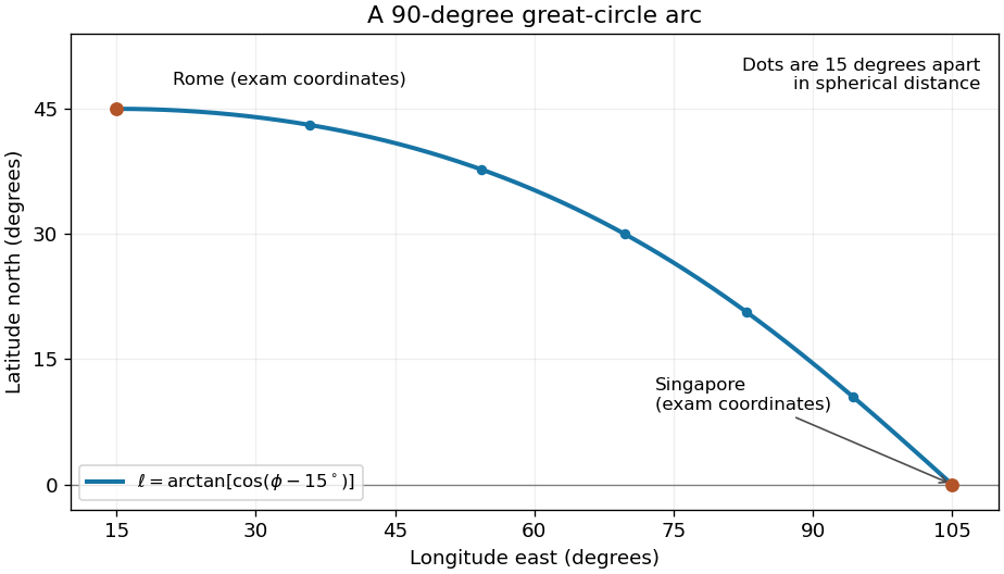
Shortest spherical route for the approximate Rome and Singapore coordinates in the question
. Latitude versus longitude for the derived great circle, with endpoints at 45 degrees north and 15 degrees east, and zero degrees north and 105 degrees east. The quarter-circle parameter increases uniformly in spherical distance. Details.
For an explicit regular arc-length parametrization, let and . Their dot product is . HenceBoth and equal one. The shorter great circle arc is the global shortest path: for any unit-speed curve from , its central angle satisfies by the Cauchy-Schwarz inequality, since the tangential projection of has length . Integrating gives length at least the endpoint angle , which this route attains. For a sphere of radius , the corresponding shortest distance is .
Articles by others on the same topic
There are currently no matching articles.