The weight cancels the denominator in the Sturm-Liouville operator. Two integrations by parts, with real , give the Lagrange identity for a Sturm-Liouville operatorThus the boundary form must vanish for every pair in the operator domain:Separated real Robin boundary conditions at , with , make each endpoint contribution vanish. This includes Dirichlet boundary conditions and Neumann boundary conditions. Coupled conditions can also work: periodic and cancel the two endpoint contributions. For the regular problem, imposing a complete pair of such self-adjoint boundary conditions gives a self-adjoint differential operator; the displayed identity is the boundary-form criterion.
First, setting in the self-adjoint operator identity shows that is real, so every eigenvalue is real. For two eigenfunctions,Distinct eigenvalues therefore implyThis is orthogonality of Sturm-Liouville eigenfunctions.
Factor out from the differential expression:Comparing with givesMultiplying all three by the same positive constant would give the same Sturm-Liouville operator.
Use a logarithmic change of variable in a Sturm-Liouville problem: set and . The chain rule givesThe endpoint conditions become . Multiplying by and integrating shows that for a nonzero solution. Put . The first endpoint selects and the second requires , . HenceThese eigenfunctions are orthonormal in the specified weighted inner product, because and
Expand the solution and the forcing in the orthonormal Sturm-Liouville eigenfunction expansion. The forcing coefficients areEvery is nonzero, so the solution coefficient is . ThusAs an independent check, solving directly with the two endpoint conditions givesIt satisfies both Dirichlet boundary conditions and the forced ordinary differential equation.
A single-valued potential must be -periodic in . For a separated solution , the Laplace equation in polar coordinates becomesThe periodic angular eigenvalue problem has , : its nonconstant eigenfunctions are . Negative gives exponentials that cannot be periodic, and gives only a constant angular factor. For , the radial Cauchy-Euler equation gives . At the two radial solutions are and . Superposition therefore givesThe expansion is interpreted on an annulus where the harmonic function is defined; particular boundary conditions determine its constants and convergence region. Single-valuedness is essential: allowing a cut in the angular domain would also permit nonperiodic angular solutions.
Treat each angular Fourier mode independently. Boundedness at the axis excludes the negative radial powers and the logarithm inside; decay at infinity excludes the positive powers, constant and logarithm outside. For the cosine mode writeContinuity at gives . The jump of the normal derivative is thenThus and . The sine mode has the same relation with . Therefore the potential of a charged cylindrical shell with angular Fourier data isThere is no angular mean term: the given surface charge density has zero average. The interior constant is zero because its boundary value must match the vanishing exterior mean. A nonzero mean charge per unit length would instead produce a logarithmic electrostatic potential, incompatible with the specified decay at infinity.
Apply the product rule to the vector field :The gradient cross terms cancel. Integrating and applying the divergence theorem with outward unit normal proves Green's second identity:Choose the Dirichlet Green function with and on . Taking and using the Dirac delta distribution, the left side becomes while the second boundary term vanishes. HenceThe plus sign is tied to the convention , whose free-space fundamental solution is negative in three dimensions. The singularity may equivalently be handled by excising a small sphere about before applying the smooth identity.
Put . Away from the source, the radial Laplacian in three dimensions givesThus . At the source it is a distribution, not a smooth function; its outward gradient flux through a small sphere is , giving .
Write and . If , expansion of squared Euclidean distances givesConsequently , and the two terms in cancel. This method of images gives the Dirichlet Green function inside a sphere:The image point is outside the sphere, so only the physical source contributes a Dirac delta distribution inside. As , the image position tends to infinity and its coefficient also diverges, but their ratio has the finite limitThusThe apparent singularity of the image construction at a central source is removable; the physical source singularity at remains.
Let be the reflection of the source in the equatorial plane. For a source in the upper half-ball, the Dirichlet Green function inside a hemisphere isBoth terms vanish on the spherical boundary. On the flat boundary , the two source distances are equal, and the distances to their spherical image points are also equal, so the difference vanishes there too. The reflected physical source is in the lower half-ball and both inverted image points are outside the sphere. Therefore the only source singularity in the desired region is the original one, with coefficient in . This combines reflection with the spherical method of images.
Reflecting repeatedly in the two parallel planes creates an infinite method of images. For , introduceThe Dirichlet Green function between parallel planes isEach bracket is , so the paired series converges absolutely away from the sources. At , reflection pairs the positive image indexed by with the negative image indexed by . At it pairs that positive image with the negative image indexed by . The distances agree in each pairing, making both boundary values zero. This can be checked with symmetric finite partial sums first; the unmatched end terms tend to zero, so no subtraction of separately divergent series is needed. Only lies within the slab, so . This is the usual Green function decaying at large transverse separation; such a condition selects the physical solution in the unbounded region.
A function is an analytic function at if it is holomorphic throughout some open neighbourhood of , equivalently if it has a convergent power series there. In real components , continuous first partial derivatives in a neighbourhood together with the Cauchy-Riemann equationsthroughout that neighbourhood are sufficient, and for an analytic function they hold there. Satisfying these equations only at the single point is not enough to establish analyticity in a neighbourhood.
Factor the polynomial denominator as . The numerator has values and at the two roots, so neither cancels. ThereforeThe factor gives a branch point at zero, with local behaviour . Infinity is also a branch point, since in the coordinate the leading behaviour is . A single-valued branch requires a branch cut joining these points. Away from that cut and the two poles, the selected branch is holomorphic. For the integral below, use , putting the cut along the positive real axis.
Use a counterclockwise keyhole contour around the positive real branch cut, with small radius and large radius . On the upper bank , so the integral tends to . On the lower bank , , giving the negative of the upper-bank integrand. That bank is traversed from to , so its contribution also tends to .
The outer circle contributes , since and its length is . The small circle contributes , since . Both vanish. HenceThe contour encloses both double poles but excludes the branch point.
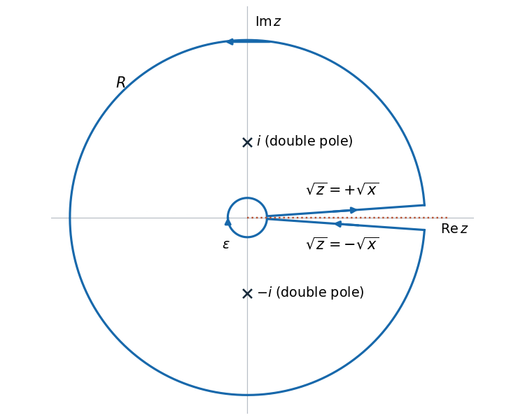
Keyhole contour around the positive real branch cut
. The upper bank runs outwards and the lower bank runs inwards. The large circle is counterclockwise and the small circle is clockwise; both poles lie inside the contour. The gaps are enlarged for visibility. Details.
For a double pole at , differentiate the remaining holomorphic factor:Since and , this simplifies toOn the selected branch and , givingThe residue theorem therefore givesThe equality uses the limiting contour integrals established in (c).
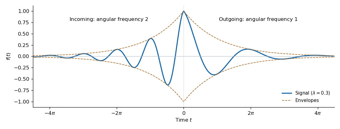
The signal is continuous at zero with . Its envelope is , but its angular frequency falls from on the incoming side to on the outgoing side. Its one-sided slopes are and , producing a cusp at the peak. Both tails decay to zero.

Use . Expanding each cosine into two exponentials and integrating its half-line givesEquivalently,The positive guarantees convergence of the Fourier transform integrals.
The Fourier transform of a derivative gives . For ,This selects the solution decaying at both time infinities. Indeed, the inverse transform of is the one-dimensional modified Helmholtz Green function , and the convolution theorem gives . The printed equation has homogeneous solutions , so these two decay conditions matter; no causal initial-value condition was specified.
For , evaluate Fourier inversion by closing the contour in the lower half-plane, where decays. The contour is clockwise. The enclosed simple poles and residues of areThus inversion equals times the sum of the residues of , givingAs a check, applying gives . The convolution also gives for ; the two pieces have matching values and matching first derivatives at zero.
Under an orthogonal matrix , the Levi-Civita symbol satisfiesUse this twice, and use for the contracted index. It follows thatTherefore : it is a fourth-rank isotropic tensor. Although a single alternating symbol is a pseudotensor under reflections, the two determinant factors multiply to one, so this product is an ordinary tensor even for improper orthogonal transformations.
Use three components of the proposed isotropic tensor form. Since , one gets . Since , one gets . Finally gives . Hence contraction of two Levi-Civita symbols gives
The integration domain is invariant under every rotation matrix, and its volume element is unchanged. The substitution therefore provesThus is an isotropic tensor. It is also completely symmetric in its four indices, because the coordinate factors commute. In the general isotropic form, exchanging indices equates and , and exchanging equates and . Therefore
Contract the isotropic expression from (i). Since and ,The value in (ii) gives , so the isotropic fourth moment of a ball isFor example and , illustrating the factor of three between these two fourth moments.
Write the inverse tensor asInsert this into and equate powers of . One obtains successivelyThus the Neumann series givesEvery contraction is an ordinary ordered matrix product. No transpose or symmetry assumption is used. Multiplying the truncated series on either side by leaves , which verifies the error order. For a fixed finite matrix this expansion converges whenever in a submultiplicative matrix norm.
For the stated square side length , the volume is and the uniform mass density is . Direct integration about its central vertical axis gives the moment of inertia of a uniform square plate:Thus the PDF's coefficient is inconsistent with its stated side length. The coefficient would apply to a square of side .
For the disc, use cylindrical coordinates and :For the sphere, use spherical coordinates and :These agree with the moment of inertia of a uniform disc and the moment of inertia of a uniform solid sphere. The square's thickness does not enter its axial moment of inertia once the mass is fixed.
Measure each generalized coordinate from an unstressed configuration. The diagram has one torsional spring joining the frame to object 1, one joining objects 1 and 2, and one joining objects 2 and 3. The rotational kinetic energy and elastic potential energy areEach spring contribution follows by integrating its restoring torque: . ThusThe Euler-Lagrange equations giveThese hold for either interpretation of the square's moment of inertia; the geometry-based value from (a) is used first below.
For the stated geometry and numerical masses, the inertia and stiffness matrices areA normal mode requires . Writing , its characteristic equation isAt the claimed , this determinant is . Hence the printed claim that is a normal frequency is false for the stated data, and there is no corresponding nonzero normal mode.
The complete geometry-based answer is obtained from the three positive roots :An exact closed form for the squared angular frequencies isThey are approximately , and , respectively. For any of these roots, a corresponding eigenvector can be chosen asThe last two rows of give this expression directly; the first is the characteristic equation. These three modes span all motion, with arbitrary sine and cosine amplitudes. Positivity of and of the spring potential energy ensures that all squared angular frequencies are positive.
If instead one takes the PDF's printed as a stipulated inertia, then andThe corresponding angular frequencies are approximatelyThe same formula for applies, because its derivation used only the second and third rows. Here the determinant at is , so following the printed inertia does not repair the frequency claim. The PDF therefore needs a further correction to its numerical data or asserted frequency; the intended correction cannot be inferred uniquely.
Subtraction fails associativity: but . Thus it violates the group axioms and is not a group. It has a right identity , but no element can be a two-sided identity element.
The operation is not defined for every pair in the proposed set: choosing makes its denominator zero. Thus it is not even a binary operation on , and is not a group. In particular, removing zero from the domain does not prevent the sum in the denominator from vanishing.
The substitution , with , is a bijection onto and obeysThus the log-sum-exp function transfers nonnegative addition to the given set. It is closed, associative and commutative, with identity element . But a finite has , and adding a nonnegative number cannot give zero, so no finite has an inverse element. Therefore it is a commutative monoid but not a group.
The sum of two odd integers plus one is odd, so the operation is closed. Both associations of a triple give , proving associativity. Its identity element is , and the inverse element of is , also odd, since . Thus it is an abelian group.
More explicitly, shifted addition on odd integers is ordinary integer addition in different coordinates:This bijection is a group isomorphism to .
For a subgroup and , the left and right cosets are and . A normal subgroup satisfies for every . Multiplying this set equality on the right by givesConversely this equality implies , so it is an equivalent definition of normality.
For a normal subgroup , the quotient group consists of its cosets with multiplicationTo check that this is well-defined, replace by with . Their product issince normality puts in . Hence the product does not depend on representatives. Associativity follows from that in , the identity element is , and . These verify the group axioms.
Lagrange's theorem counts the equal-sized cosets:Finally, if is prime, choose . Its cyclic subgroup has order greater than one dividing , hence equals . All elements are powers of , so . Thus
Write a matrix in the set as . The zero matrix has no multiplicative inverse matrix, so is not a group. Its determinant iswhich vanishes only at that zero matrix. It is therefore the only element that needs to be removed.
For closure, direct matrix multiplication givesThe product of nonzero determinants is nonzero, so two nonzero elements never multiply to zero. The identity matrix is , associativity is inherited from matrix multiplication, andThus . It is the multiplicative group of nonzero quaternions in the complex matrix representation of quaternions.
Act on the four labelled vertices. A proper rotation gives an even permutation, identifying the rotational tetrahedral symmetry group with , an alternating group. Geometrically there are one identity, three half-turns about opposite-edge midpoint axes, and two nontrivial rotations about each of four vertex-face axes. ThereforeThe tetrahedral rotation conjugacy classes areTo justify the splitting, the centralizer of a 3-cycle within is its three-element cyclic subgroup, so its conjugacy class has size . Its inverse is not conjugate to it in : the permutations that reverse that cycle while preserving its fixed vertex are odd. Conjugating by the even permutations produces the displayed , and taking inverses gives . The three half-turns are conjugate, since rotations move their axes into one another. Their centralizer has order four and their class therefore has size three.
LetThe product of any two distinct nonidentity elements is the third, and each squares to , so is a Klein four-group. Conjugating a double transposition simply relabels its letters, keeping it in the set. Hence is a normal subgroup of .
Choose . The cosets are distinct and cover the twelve elements. With , defineThe coset decomposition makes this well-defined. Normality givesso preserves products. It is onto , andThis is the tetrahedral quotient onto the cyclic group of order three. In terms of (a), it sends to , to , and to . The normality check above also follows abstractly because a group homomorphism kernel is normal.
The group is the direct product of groups . Repeatedly adding returns to for the first time when both and divide the step number. Its order of a group element is therefore . If are coprime, this is , so it generates every element:Explicitly, is the Chinese remainder theorem group isomorphism.
If , every pair satisfiesThus every element order divides , and no element can generate the whole group. HenceThis is the cyclicity of a product of two finite cyclic groups.
The upper-left block of is the planar rotation matrix , and fixes the third coordinate. ThereforeThe diagonal entries of square to one, so . Direct conjugation gives , hence for every integer . ConsequentlyWhen , the last exponent is four, which is equivalent to zero because .
The relations in (a) reduce every word in the generators to , with and . These eight matrices are distinct: the elements have third diagonal entry and the elements have entry , while the four planar blocks are distinct in each family. Their multiplication iswith exponents reduced modulo four and two. This proves closure. The identity element is , the inverse of is , and each is its own inverse. Associativity is inherited from matrix multiplication, proving the group axioms. This is the eight-element dihedral group .
Set and for , consistently with the two labels specified in the question. The row-times-column multiplication table isThe rotation powers commute with one another, and commutes with exactly when is even. Two elements commute exactly when is even. These statements also check the symmetric portions of the table.
The character of a representation is the trace of its representing matrix. For the rotation powers,Each has a planar reflection block of trace zero and third diagonal entry , giving character . In the chosen element order,Equivalently its values on the conjugacy classes , , , , are .
The complete subgroup list isThus there are ten subgroups: one trivial, five of order two, three of order four, and the whole group. The five order-two subgroups are mutually isomorphic. The two noncyclic order-four subgroups are mutually isomorphic Klein four-groups; neither is isomorphic to the cyclic group of order four.
For completeness, Lagrange's theorem permits only orders . An order-four subgroup containing or must be . Otherwise it can contain only and elements . The product of two distinct such elements is . To avoid generating or , their exponents must differ by two, giving exactly the two listed Klein four-groups. The order-two subgroups come from the five involutions and . This proves completeness.
Articles were limited to the first 100 out of 101 total.
Articles by others on the same topic
There are currently no matching articles.