For a continuously differentiable vector field on a bounded region with piecewise smooth closed boundary , the divergence theorem statesHere is its divergence, is the volume element, is the surface area element, is the outward unit normal, and . Thus a volume integral of the divergence equals the outward flux through the boundary.
Since is constant, the product rule gives . Applying the divergence theorem therefore givesThis holds for every constant vector , so each component of the difference vanishes. Consequently the gradient has the boundary representation
The divergence of a cross product and give . On the boundary the scalar triple product gives . Thus the divergence theorem givesBecause is arbitrary, the curl identity follows:
Use Einstein summation convention and write . Since , where is the Kronecker delta, the product rule givesThis proves . Now take . Integrating this identity and applying the divergence theorem to the first term givesPart (b) changes the last volume integral of the gradient into a surface integral, yieldingHere ; the Laplacian is .
Apply the product rule to the tensor field, without assuming any symmetry of :Integrating, the divergence theorem converts each of the two divergences into a boundary term:The repeated indices are summed according to Einstein summation convention, while labels the component of the resulting vector identity.
Choose the symmetric tensor fieldThe product rule and equality of mixed partial derivatives giveThis is the Euclidean scalar-gradient stress identity. Substitute it into part (e), and use , where . Reassembling the components gives the required pure surface integral:Sufficient smoothness of is understood for the displayed derivatives and applications of the divergence theorem.
Apply separation of variables with and temporal factor . The spatial eigenvalue equation isThe nontrivial solutions of these Dirichlet boundary conditions are sine eigenfunctions. Normalizing in the usual inner product on giveswith . The superposition principle and the Fourier sine series then giveThe constants are the initial-data coefficients . Here physical diffusion means .
By orthogonality and the sampling property of the Dirac delta distribution,Consequently the reaction-diffusion equation solution isFor every this eigenfunction expansion is smoothed by the Gaussian decay in . As , it recovers the specified initial condition in the sense of distributions.
The smallest decay-rate eigenvalue is , so the threshold isBecause , . For every fixed interior point , the first sine eigenfunction is positive and the remaining terms have strictly faster decay relative to it. HenceOne can justify the relative-error limit directly: after factoring out the first exponential, the absolute remainder is bounded by , which tends to zero. Thus , and . The boundary values stay zero. At equality the first term is stationary and the density approaches its positive sine profile.
Let . The first normalized Fourier sine series coefficient isStrict positivity follows because , has positive total mass, and everywhere inside the interval. In particular, there is no cancellation that could remove the slowest term. This is the positivity of the first Dirichlet reaction-diffusion coefficient.
For finite initial mass , all coefficients satisfy . The eigenfunction expansion therefore gives the uniform boundThe positive first profile thus controls the long-time behavior. We recover exactly the threshold , with decay below it and unbounded positive growth at every interior point above it. The finite-mass condition is the usual meaning of an initial density profile here; standard positive-time smoothing gives the same conclusion in the usual broader admissible data classes.
For an exponential trial , the characteristic equation isIts distinct complex roots are . Thus the general real solution of the homogeneous second-order linear differential equation isThe two displayed solutions have nonzero Wronskian and hence linear independence. The same formula permits complex solutions when are complex.
For the zero-data initial value problem, choose a causal Green function satisfying and for . Continuity at prevents a derivative of the Dirac delta distribution, while integration across the source givesFor , part (i) gives the shifted homogeneous solutions. The zero value at the join removes the cosine term, and the unit derivative jump fixes the sine coefficient. Therefore the causal Green function of a damped oscillator isEquivalently, multiply the first expression by the Heaviside step function . The required solution isIts initial value and first derivative vanish: the interval has zero length at and the kernel vanishes at its upper limit. Differentiating twice shows that the upper-limit contribution to is precisely , while the remaining homogeneous kernel terms cancel in .
The original PDF has the absolute-value hypothesis , which is missing from the local OCR. From the Green's function formula and ,Because , the upper bound tends to zero. The squeeze theorem proves .
With the paper's Fourier transform convention, the Fourier inversion theorem givesThis holds at continuity points under the usual inversion hypotheses; at a jump with one-sided limits it gives their mean. The factor and the sign change in the exponential are part of this normalization.
Insert the inverse Fourier transforms of and its complex conjugate, initially under enough decay to justify interchanging integrals:The middle step uses the stated Dirac delta distribution identity, and the last uses its sampling property. This is the Parseval identity for the chosen normalization. Approximation extends the result to square-integrable functions, including the function used below.
The real odd function has a purely imaginary odd Fourier transform. Setting and using a product-to-sum identity,The apparent singularities are removable. Direct evaluation or limits giveIn particular, the transform stays finite where its numerator and denominator both vanish.
The squared norm of the original function isApplying the Parseval identity to part (c), using the evenness of the squared transform, givesThus the last integral equals . Now set . Sincewe obtainThe apparent singularity at is removable: the continuous value of the integrand there is . No principal-value interpretation is needed.
Let with . Taking the Hermitian inner product with gives . For an anti-Hermitian matrix,Consequently . As , the eigenvalue satisfies , or . Zero is included as a purely imaginary eigenvalue.
If were a singular matrix, a nonzero vector would satisfy , so . This would make an eigenvalue of the anti-Hermitian matrix, contrary to part (a). Thus . The same argument shows is an invertible matrix, which will also be used below.
Taking the conjugate transpose term by term in the convergent matrix exponential givesThe matrices and commute, so the matrix exponential product law gives and likewise . Hence .
For , use the inverse and product rules for the conjugate transpose:The factors commute, as do their inverses, since they are expressions in the same matrix. Consequentlyand similarly . Therefore . This rational construction is the skew-Hermitian form of the Cayley transform of a Hermitian matrix, obtained by writing with a Hermitian matrix.
If , then , and the matrix exponential series gives . Also , since . ThusThe assumed diagonalization ensures that these account for all eigenvalues, including multiplicities. In particular, for ,both of modulus one, in agreement with the unitary matrix property.
Here . Splitting the matrix exponential into even and odd powers therefore givesFor the second matrix, , so . HenceBoth are real orthogonal matrices, and hence also unitary matrices.
Choose a real unit eigenvector of the real symmetric matrix , with eigenvalue . Its orthogonal complement is an invariant subspace: for any with ,The restriction of to this -dimensional space is again real and symmetric. Applying the same argument inductively produces an orthonormal basis of real eigenvectors. The base case is immediate. This proves the spectral theorem for real symmetric matrices without assuming that distinct eigenvalues are available.
One can also check that eigenvectors with different eigenvalues are automatically orthogonal: . Within a repeated eigenspace, the Gram-Schmidt process preserves the eigenvector property. Thus repeated eigenvalues cause no obstruction, and .
The quadratic form is for the real symmetric matrixThe axis has eigenvalue . On the plane, the characteristic polynomial isThus the orthogonal diagonalization from part (a) yieldsFor later use, one possible orthonormal basis isThen , , . This explicit choice also confirms that the Euclidean norm is preserved: .
In the orthonormal basis of part (b), the three quadric surfaces have the following forms. For ,a two-sheeted hyperboloid with axis , vertices , and one sheet on each side of the plane . For ,an elliptic cone with vertex at the origin and the same axis. For ,a one-sheet hyperboloid with axis and a waist ellipse at , whose semiaxes are along and along . The sections at fixed enlarge away from the waist.
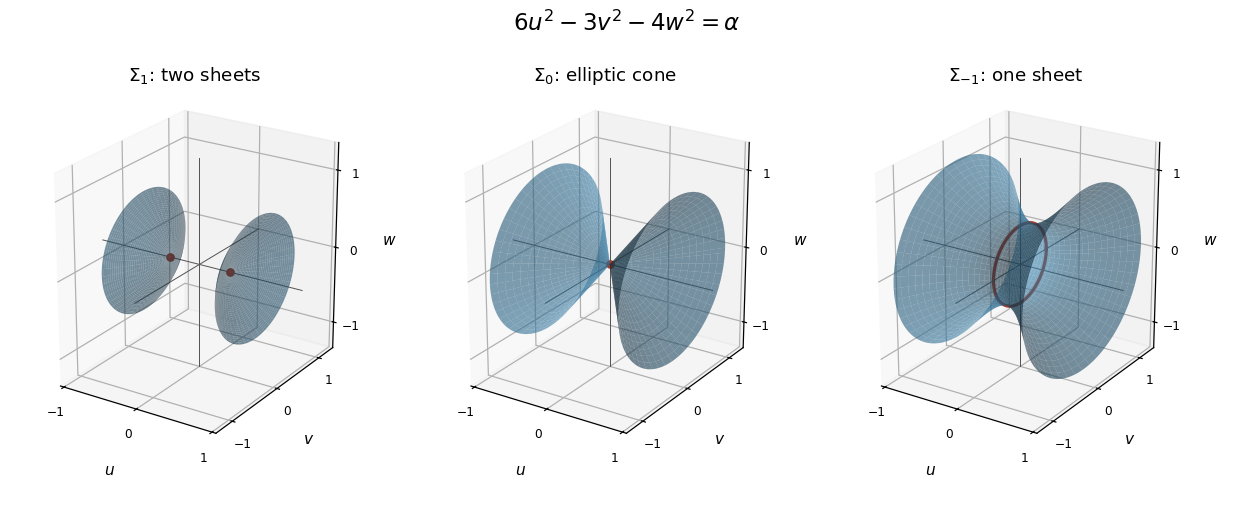
The two-sheeted hyperboloid, elliptic cone and one-sheet hyperboloid in separate orthonormal coordinate frames
. Details. 
The orthogonal change of coordinates preserves distance to the origin. On the required quadric surface,Thus the squared distance is at least . Equality holds precisely when , and the constraint then gives . Using from part (b), the nearest points in the original coordinates areSubstitution checks the constraint directly: . The inequality proves these are global nearest points, rather than merely stationary candidates.
Write and square the modulus equation. It becomesFor , completing the square gives the Apollonius circleHenceThe printed statement needs the exception : equal distances from and give their perpendicular bisector, a straight line rather than a finite-radius circle. For the center lies in the upper half-plane; this is the case needed in part (ii). The original PDF confirms the numerator , correcting the duplicated, corrupted OCR formula.
For the upper Apollonius circle, let its constant ratio be . Matching the center and radius from part (i) givesSubtracting their squares yields . AlsoThe relevant inverse hyperbolic cosine is positive. Now is the real part of a local holomorphic logarithm, hence a harmonic function away from . The point is inside the excluded disk, because , while is below the real axis. Thus neither singularity lies in the physical domain.
On the numerator and denominator have equal modulus, so the logarithm is zero. On the circular boundary its value is . Therefore the harmonic potential between a grounded line and a circular boundary isThis verifies Laplace's equation and both prescribed Dirichlet boundary conditions. It also tends to zero at infinity. A uniqueness assertion on this unbounded domain would require an additional boundedness or infinity condition; the displayed function is the natural decaying solution requested.
Substituting into the defining Gamma integral givesBoth endpoints are convergent, so no continuation of the Gamma function is needed here.
For real , apply integration by parts to the Gamma integral with and :The boundary term vanishes: at zero, and exponential decay dominates the power at infinity. This proves the Gamma function recurrence
Iterating the Gamma function recurrence gives a meromorphic continuationNear , the numerator is analytic and tends to . Exactly one denominator factor, , vanishes, while all other factors tend to the nonzero product . ThereforeThus . More precisely, the Gamma function residue at a nonpositive integer is . Taking large enough to put in the original right half-plane also shows that this continuation introduces no other finite poles.
First simplify the coefficient of usingAfter dividing by , the second-order linear differential equation isAt zero, and , and both products are analytic there. At , and , again with analytic extensions. Thus , and there are no other finite singular points.
Infinity must also be considered because the question asks for all singular points. Put and . The coefficient of in its normal-form equation is . Multiplication by does not make it analytic at zero. Hence .
Set and use the Frobenius solution with . From part (a), the leading coefficients are and . The coefficient of the lowest power is thereforeThe indicial equation reduces to , givingSince , the two indicial roots differ by a nonzero imaginary number, not an integer. Thus the two local Frobenius solutions exist independently on a chosen branch of .
Define the Wronskian by . Differentiating and using the normal-form differential equation givesIntegrating this first-order linear differential equation proves Abel's identity:Thus, on any interval avoiding zero and ,Absolute-value signs from real logarithms can be absorbed into the constant on each such interval. For linearly independent solutions, .
At zero the indicial equation is , with repeated indicial root zero. To exhibit the analytic solution rather than only its candidate exponent, clear the denominator in the normal form:Substitute and equate coefficients. With for negative indices, the linear recurrence relation isEvery leading coefficient on the left is nonzero. Hence is free and all later coefficients are determined; the Frobenius method guarantees local convergence up to the next singularity. In particular,For a second solution, use reduction of order. Writing gives , so part (c) yieldsThe additive constant in the integral only adds a multiple of . As within , its integrand isThereforeThe nonzero Wronskian proves linear independence, and the logarithm is unavoidable for this second local solution.
For fixed initial and final coordinates, the two Euler-Lagrange equations areIndeed the first variation of the functional isIntegration by parts moves the time derivatives from the variations; their endpoint values are zero. The fundamental lemma of the calculus of variations then gives the two equations above.
The total derivative contributes only the boundary termThis is fixed by the endpoint data, so its first variation vanishes. It cannot change the Euler-Lagrange equations or which path minimizes .
For a direct check, let . ThenThe equality uses commuting mixed partial derivatives. Thus , as in total time derivatives preserve fixed-endpoint Euler-Lagrange equations.
This is an isoperimetric constraint, imposed on the whole path rather than separately at each time. Introduce a constant Lagrange multiplier and replace the variational integrand by . The modified Euler-Lagrange equations areSolve these together with the fixed endpoint conditions, treating as an unknown constant, then choose its value so thatThe multiplier is constant because there is one scalar integral constraint. A condition imposed at every time would instead call for a time-dependent multiplier. As usual, this multiplier procedure assumes the constraint is regular, so its first variation does not vanish identically on all admissible variations.
The needed partial derivatives areSubstitution into the Euler-Lagrange equations givesThe terms cancel in the first equation, leavingThese are accompanied by and . The cancellation is consistent with part (b): the term proportional to is the total derivative of .
Impose before varying. Writing , the restricted integrand isIts middle term is the total derivative of , so it can be dropped for fixed endpoints by part (b). The remaining Euler-Lagrange equation is . Integrating twice and imposing , givesThis is the unique global minimizer among paths on the specified line. To prove it, add any admissible variation with . The change in fuel, after dropping the fixed boundary term, isThe first integral vanishes by integration by parts and the equation for . Equality forces . No monotonicity or restriction to the segment between endpoints was imposed in the question; the minimizing coordinate can initially decrease for sufficiently large .
Use the standard regular Sturm-Liouville problem hypotheses: positive weight , real coefficients, and real self-adjoint boundary conditions. The positive weight and boundary-domain assumptions are implicit in the requested real orthonormal basis; real differential coefficients alone would not guarantee them for arbitrary complex boundary conditions.
Multiply the eigenfunction equation by and integrate. By self-adjointness, the number is real, whereasThe second integral is strictly positive, so . Because the coefficients and boundary conditions are real, the real and imaginary parts of any complex eigenfunction separately obey the same equation and conditions. At least one is nonzero, so a real eigenfunction can be chosen. More generally, each eigenspace has a real basis, which can be orthonormalized using the weighted inner product.
The orthogonality of Sturm-Liouville eigenfunctions, with normalization chosen to one, isFor the real choice, omit the complex conjugate.
The Sturm-Liouville eigenfunction expansion of a suitable real function isComparing this identity with the sampling property of the Dirac delta distribution gives the completeness kernelThis is an identity of distributions, rather than a pointwise-convergent series of ordinary functions.
Assuming zero is not an eigenvalue, define the spectral Green function of a regular Sturm-Liouville problem byApplying gives : multiplying the preceding completeness kernel by leaves the Dirac delta distribution unchanged. Each term also obeys the same homogeneous boundary conditions. There is no extra weight factor in for the ordinary source measure .
If zero is an eigenvalue, the inverse Green's function does not exist on all forcing functions: the forcing must obey the solvability condition at a Sturm-Liouville eigenvalue. Omitting the zero mode instead constructs a reduced inverse, with its projection removed from the right-hand side. This exception occurs in part (c) at .
Write the endpoint condition in its linear Robin boundary condition form . For a positive eigenvalue , the left Dirichlet boundary condition gives , and the right condition givesFor each positive root , the squared norm isConsequently the sine coefficients in any complete expansion areWhen , these are all modes and the Sturm-Liouville eigenfunction expansion gives exactly the stated sine series, with the usual convergence interpretation. Positivity of all eigenvalues follows from integration by parts and the Cauchy-Schwarz inequality:for a nonzero admissible , since .
However, the original PDF states only , and with that range its sine-only completeness claim is false. The missing modes are as follows. At , admits , so the correct expansion isFor , a negative eigenvalue admits , withThere is exactly one positive root: decreases strictly from to zero. For example, its derivative has the sign of , because . Thus the corrected expansion isThese are the nonpositive modes in a Dirichlet-Robin interval expansion. As an explicit counterexample to the printed claim, at take : it satisfies both boundary conditions, and each positive root obeysbecause . Thus all vanish despite . Likewise is a counterexample for , by orthogonality of Sturm-Liouville eigenfunctions with distinct eigenvalues. The formulas above give the full solution without silently assuming away the omitted modes.
Articles were limited to the first 100 out of 194 total.
Articles by others on the same topic
There are currently no matching articles.