Past exam of the quantum physics course of the University of Oxford / 2016 (A10431W1, A3)

Source paper: www.whatdotheyknow.com/request/physics_past_exam_papers_2015_16/response/973997/attach/3/Cowell%20Attachment.zip?cookie_passthrough=1 (member: Finals papers/A10431W1_A3_2016.pdf). The dated cover identifies the ordinary Part A sitting of 17 June 2016. All optional questions are included below. Lettered scopes separate successive marked blocks where the source leaves them unlettered.

Insert hydrogen energy eigenstates on either side of the commutator. Because $L_z$ is Hermitian and has eigenvalue $\hslash m$,ThusThis is a necessary electric-dipole selection rule, not a sufficient condition for a nonzero matrix element. For example, $⟨200|z|200⟩=0$ by parity even though $m=m^{\prime }=0$. The angular factor $z=r\cos \theta$ additionally requires $l^{\prime }=l\pm 1$: multiplication of a spherical harmonic by $\cos \theta$ gives only harmonics with the same $m$ and adjacent $l$. The commutator alone establishes only the magnetic quantum number restriction; radial integrals and the remaining electric-dipole selection rules for hydrogen must still be considered.

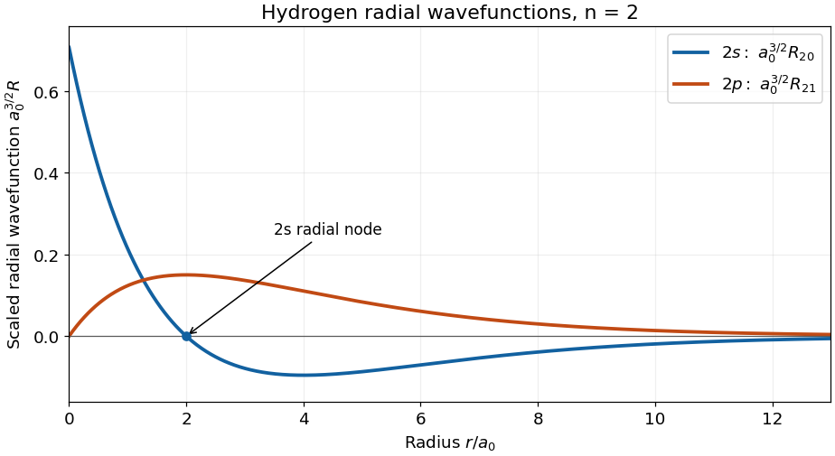
Separation of variables in the central Coulomb potential gives ${\psi }_{nlm}=R_{nl}(r)Y_l^m(\theta ,\varphi )$. The radial wavefunction depends on $n$ and $l$, independently of $m$. For the hydrogen radial wavefunction in the first excited shell, put $\rho =r/a_0$. The Bohr radius is $a_0=4\pi {ϵ}_0{\hslash }^2/(\mu e^2)$, where $\mu$ is the electron–proton reduced mass. Choose the real phasesNear the origin, $R_{20}\to 1/(\sqrt{2}{a}_0^{3/2})$, whereas $R_{21}\sim r/(\sqrt{24}{a}_0^{5/2})$. More generally, regular hydrogen radial wavefunctions behave as $r^l$. At large $r$, both displayed functions have a polynomial factor proportional to $r$ multiplying $e^{-r/(2a_0)}$; $R_{20}$ approaches zero from below and $R_{21}$ from above with these phase choices.

The $2s$ radial wavefunction crosses zero once, at $r=2a_0$, and has its negative minimum at $4a_0$. The $2p$ radial wavefunction has no radial node at positive $r$, and reaches its maximum at $2a_0$. The count is $n-l-1$; neither the origin nor the limit at infinity is counted as a radial node. These are sketches of $R$, rather than of $rR$ or the radial probability density $r^2|R{|}^2$.

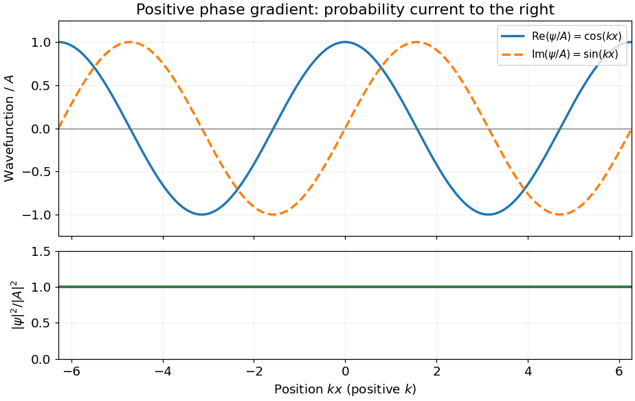
For the Schrödinger equation with a real scalar potential and no vector potential, the probability current isTogether with the probability density $\rho =|\Psi {|}^2$, it satisfies the continuity equation ${\partial }_t\rho +\nabla \cdot \mathbf{j}=0$. Substituting ${\partial }_x\Psi =ik\Psi$ givesA complex wavefunction requires both its real and imaginary parts in the sketch. Choosing the irrelevant constant phase so that $A$ is real, they are $A\cos kx$ and $A\sin kx$, while the probability density is horizontal. It is the spatial phase gradient of a Schrodinger wavefunction ${\partial }_x\arg \Psi =k$ that determines the sign of the probability current. In particular, $e^{ikx}$ and $e^{-ikx}$ have the same real part but opposite probability currents, so the slope of the real part cannot determine the direction.

A nonzero plane wave on the whole real line is not square integrable. The displayed density is understood with box normalization, generalized normalization, or as a local description of a broad wave packet; it does not define a normalized probability distribution on the whole line.

Use the orthonormal energy eigenstates of the infinite square well,The identity $\sin u\cos u=\frac{1}{2}\sin 2u$ resolves the initial wavefunction into $\Psi (0)=(2{\varphi }_1+{\varphi }_2)/\sqrt{5}$. Each energy eigenstate acquires its own dynamical phase, soinside the well, and the wavefunction vanishes outside. The energy probabilities are $4/5$ and $1/5$ at every time. ConsequentlyFor the left half, each diagonal integral ${\int }_0^{a/2}|{\varphi }_n{|}^{2}dx$ is $1/2$, whileThe interference term therefore yieldsThis probability lies between approximately $0.1605$ and $0.8395$, with period $2\pi \hslash /(3E_1)$. A conserved energy distribution is compatible with time-dependent position probabilities because the relative quantum phase keeps evolving.

Identify the nonrelativistic mass with the rest mass, $m=m_0$. Expanding the relativistic kinetic energy in $p^2/(m^2{c}^2)$ givesFirst-order perturbation theory requires $\Delta E_0=⟨0|H^{\prime }|0⟩$. Put $\alpha =\sqrt{m\hslash \omega /2}$, so $p=i\alpha (a^{†}-a)$. The annihilation relations are $a|0⟩=0$ and $⟨0|a^{†}=0$. In particular, $a^{†}|0⟩$ does not vanish. A short calculation retaining the operator ordering givesEquivalently, of the ordered words in $(a^{†}-a{)}^4$, only $a{a}^{†}a{a}^{†}$ and $aa{a}^{†}{a}^{†}$ have nonzero ground-state expectation values, respectively $1$ and $2$. Words with a creation operator on the far left or an annihilation operator on the far right vanish; the remaining unbalanced words also vanish. ThusThe correction is negative because the relativistic kinetic energy is smaller than $p^2/(2m)$ at fixed nonzero momentum. This relativistic oscillator ground-state kinetic correction requires $\hslash \omega \ll m{c}^2$.

For two spin one-half particles, $s_1^2=s_2^2=3{\hslash }^2/4$. Squaring $\mathbf{S}={\mathbf{s}}_1+{\mathbf{s}}_2$ givesTake $a,b$ real so that $f$ is Hermitian. Since $[S^2,S_z]=0$, the displayed polynomial implies $[f,S^2]=[f,S_z]=0$. There is a common orthonormal eigenbasis, so all three observables can be simultaneously certain in a common eigenstate. Commutation does not mean that every quantum superposition has definite values of all three.

Suppress the fixed individual quantum numbers $s_1=s_2=1/2$. In the coupled basis, ordered on both rows and columns as $|1,1⟩,|1,0⟩,|1,-1⟩,|0,0⟩$, the total-spin eigenvalues giveHere the first three entries form the triplet state sector and the last is the singlet state. For the product basis, useThe first term has diagonal entries ${\hslash }^2(1,-1,-1,1)/4$. Each nonzero exchange term flips $|\uparrow \downarrow ⟩$ to $|\downarrow \uparrow ⟩$ or back, with coefficient ${\hslash }^2/2$. With rows and columns ordered as $|\uparrow \uparrow ⟩,|\uparrow \downarrow ⟩,|\downarrow \uparrow ⟩,|\downarrow \downarrow ⟩$,The change of basis is made explicit by $|1,0⟩=(|\uparrow \downarrow ⟩+|\downarrow \uparrow ⟩)/\sqrt{2}$ and $|0,0⟩=(|\uparrow \downarrow ⟩-|\downarrow \uparrow ⟩)/\sqrt{2}$, with $|1,\pm 1⟩=|\uparrow \uparrow ⟩,|\downarrow \downarrow ⟩$. The resulting eigenvalues reproduce the diagonal coupled matrix.

The spin Hilbert space is a tensor product of two two-dimensional spaces and therefore has dimension four. Angular momentum addition decomposes it asThese are three orthogonal triplet states and one singlet state. For identical electrons the complete wavefunction must also satisfy fermionic exchange symmetry: a symmetric triplet spin factor accompanies an antisymmetric spatial factor, whereas the antisymmetric singlet spin factor accompanies a symmetric spatial factor. If both electrons occupy the same spatial orbital, only the singlet spin factor is allowed. The four-dimensional spin space does not assert four allowed spin states for that particular spatial occupation.

Expanding the total angular momentum and replacing transverse components by ladder operators givesThe particle exchange operator obeys $P_{12}^2=I$ and $P_{12}{s}_{1\alpha }{P}_{12}=s_{2\alpha }$, with the reverse relation for index $2$. These statements also apply to the ladder operators. Exchanging the indices preserves $s_1^2+s_2^2$ and $s_{1z}+s_{2z}$; it interchanges the last two terms in $S^2$. Operators on different tensor factors commute. HenceThe full particle exchange includes the spin coordinates as well as the spatial coordinates.

Write $\Psi =(|\downarrow \uparrow ⟩+|\uparrow \downarrow ⟩)/\sqrt{2}$. Each term has cancelling $z$ components, so $S_z\Psi =0$. In the formula for $S^2$, the first three terms contribute $(3/2-1/2){\hslash }^2\Psi ={\hslash }^2\Psi$. The two ladder products exchange the two terms and contribute another ${\hslash }^2\Psi$. ThereforeThis spin state is symmetric; the accompanying spatial state must be antisymmetric for two electrons. A labelled product $|{\downarrow }_1{\uparrow }_2⟩$ alone is not an eigenstate of spin exchange: its exchanged vector is orthogonal to it. Thus it cannot supply a definite exchange symmetry when multiplied by a fixed symmetric spatial factor.

This does not prohibit opposite spins in different spatial orbitals. For example, with orthonormal orbitals ${\varphi }_a,{\varphi }_b$, the Slater determinantis a valid antisymmetric two-electron state. What fails is treating persistent particle labels as physically distinguishable identities without the required antisymmetrization.

For a conditional spin measurement of identical fermions addressing the $z$ component in one spatial mode, the Born rule givesConditioned on this result, the mode spin state is $|{\uparrow }_a{\downarrow }_b⟩$; the other outcome produces $|{\downarrow }_a{\uparrow }_b⟩$. The spin product is not a spin-exchange eigenstate. The measurement has selected an addressed mode and recorded an outcome, so this conditional spin description distinguishes the measured subsystem.

The full electron wavefunction still obeys fermionic exchange symmetry. For example, the conditional spin-up outcome in spatial mode $a$ is represented in particle coordinates byIt is antisymmetric under full particle exchange. Thus the loss of a definite symmetry of the conditional spin product does not mean that measurement turns identical electrons into distinguishable particles. If the outcome is discarded, the mode spin state is instead the equal mixture of the two opposite-spin products. The measurement must specify which spatial mode is addressed for the conditional statement to be operationally meaningful.

Hermiticity of the Cartesian angular momentum components givesThe angular momentum commutation relations $[L_i,L_j]=i\hslash {ϵ}_{ijk}{L}_k$ implyFor example, $[L_z,L_x+i{L}_y]=i\hslash L_y+\hslash L_x=\hslash L_{+}$. The two terms in $[L_x^2+L_y^2+L_z^2,L_i]$ cancel in pairs, giving the first commutator. Also $[L_{+},L_{-}]=2\hslash L_z$.

The spherical harmonics satisfyCommuting $L^2$ or $L_z$ past $L_{\pm }$ therefore givesFor a nonzero result these are the eigenvalue equations with unchanged $l$ and shifted magnetic quantum number. Taking the squared norm, using $L_{\mp }{L}_{\pm }=L^2-L_z^2\mp \hslash L_z$, fixes the conventional coefficient:At the appropriate endpoint the coefficient is zero. The zero vector is not itself an eigenstate.

There is no allowed spherical harmonic with $m=l+1$, so $L_{+}{Y}_l^l=0$. The equation $-i\hslash {\partial }_{\varphi }Y=\hslash lY$ first gives $Y=f(\theta )e^{il\varphi }$. Combining the differential expressions for $L_x,L_y$ yieldsIts annihilation of the highest-weight state becomesIntegrating $f^{\prime }/f=l\cot \theta$ gives $f=C{\sin }^l\theta$, with the constant solution included for $l=0$. HenceThe phase $e^{il\varphi }$ is single valued for integral orbital quantum number $l$; normalization fixes only $|C|$, leaving a conventional constant phase.

Direct integration over solid angle givesThus $|C|=\sqrt{(2l+1)!/(4\pi )}/(2^{l}l!)$. Choosing the usual alternating sign convention,Apply $L_{-}$ successively and divide by its ladder coefficient at each step. Explicitly,The normalization follows because the product of the squared ladder coefficients is ${\hslash }^{2(l-m)}(2l)!(l-m)!/(l+m)!$. This constructs every magnetic sublevel, including negative $m$.

Separate the center-of-mass motion from the relative motion. Two equal quark masses give reduced mass $\mu =m_q/2$. Replacing the hydrogen Coulomb strength by $a>0$ gives the Coulomb binding energies and length scaleThe factor of two in the reduced mass matters: using $m_q$ directly would double the binding energy. These are relative binding energies measured from the free quark–antiquark threshold; the rest energy $2m_q{c}^2$ is excluded.

Ignoring spin and working in the fixed quarkonium internal sector, the orbital degeneracy is ${\sum }_{l=0}^{n-1}(2l+1)=n^2$. HenceNo extra spin or colour multiplicity is being counted. The degeneracy between different $l$ at fixed $n$ is special to the Coulomb potential.

The linear confinement correction to Coulomb bound states uses $H^{\prime }=br$, and its first-order energy correction in a normalized Coulomb eigenstate is $b⟨r⟩$. Replace $a_0$ by $a_q$ in the hydrogen wavefunctions. The normalized spherical harmonics remove the angular integral, leavingFor $1s$, the integral of $r^3{e}^{-2r/a_q}$ yieldsFor $2s$, put $u=r/a_q$ and square the full radial polynomial, including its cross term:For $2p$, the same calculation givesConsequently the first two Coulomb levels become, to first order,Thus the second level splits into a singlet orbital level and a triply degenerate orbital level, with $E_{2s}-E_{2p}=b{a}_q+O(b^2)$. For the confining sign $b>0$, $2p$ lies lower than $2s$: its smaller mean radius gives the smaller positive correction. The expansion assumes these corrections and the induced couplings to other principal shells are small compared with the relevant Coulomb energy gaps; $b{a}_q^2/a\ll 1$ is the governing small parameter for fixed low $n$.

The unperturbed $n=2$ level is degenerate. The useful point is that a central perturbation is already diagonal within its usual orbital eigenbasis:Angular orthogonality removes the possible mixing of $2s$ and $2p$, and also the mixing of different magnetic sublevels. Therefore the matrix required by degenerate perturbation theory needs no further diagonalization: its diagonal entries are precisely the expectation values above. It would be incorrect to justify the calculation by claiming that the unperturbed spectrum was nondegenerate.

For $b=0$ the energy needs only $n$. For a nonzero central confinement term the energy generally needs $n,l$, but remains independent of $m$. The magnetic quantum number is still needed to specify an individual orbital eigenstate, rather than just its energy.

With $\mathbf{B}=B_0\hat{\mathbf{z}}$ and $S_z=(\hslash /2){\sigma }_z$,ThusFor $B_0>0$, spin down is the lower energy eigenstate. The negative electron magnetic moment is already accounted for in the positive coefficient multiplying $\mathbf{S}\cdot \mathbf{B}$ in the given Hamiltonian.

In the ordered basis $|+⟩,|-⟩$, the transverse magnetic field producesThe off-diagonal complex exponentials follow directly from $\cos \omega t\mp i\sin \omega t$. This matrix is Hermitian at every time.

Insert the expansion with amplitudes $c_1,c_2$ and the two unperturbed dynamical phases into $i\hslash \dot{\Psi }=(H_0+V)\Psi$. Differentiation of the explicit phases cancels $H_0$, leavingEquivalently, with $\Omega =(\omega -{\omega }_0)/2$,These interaction-picture equations conserve $|c_1{|}^2+|c_2{|}^2$. They are exact for the circularly rotating magnetic drive; a rotating-wave approximation has not been used.

Differentiate ${\dot{c}}_2=-i\gamma e^{2i\Omega t}{c}_1$ and substitute the equation for ${\dot{c}}_1$. The result isPutting $c_2=e^{i\Omega t}u$ removes the first derivative and gives $\ddot{u}+{\kappa }^{2}u=0$, where $\kappa =\sqrt{{\Omega }^2+{\gamma }^2}$. For $\kappa >0$ the general solution isThe initial spinor fixes $c_1(0)=1,c_2(0)=0$, and the first-order coupled equation fixes the second initial datum ${\dot{c}}_2(0)=-i\gamma$. Thus $A=0$, $B=-i\gamma /\kappa$, andTheir squared magnitudes sum to one. If both $\Omega$ and $\gamma$ vanish, the initial amplitudes simply remain $(1,0)$; the formulas have that continuous limit.

Source convention correction. For positive $\gamma$, the printed expression for $c_2$ lacks the factor $-i$ required by the stated basis and initial vector. A concrete test is its derivative at $t=0$: the printed expression gives $+\gamma$, whereas the Schrödinger equation gives $-i\gamma$. Multiplying only $c_2$ by a phase changes the relative quantum phase. One may change the overall phase of the entire spinor, but must then transform $c_1$ and its initial amplitude as well. The printed modulus nevertheless gives the correct transition probability.

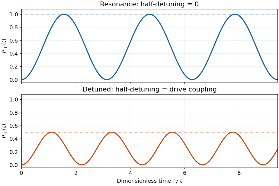
On Rabi resonance, $\omega ={\omega }_0$ and $\Omega =0$, soFor nonzero drive the probability starts at zero, reaches unity at $t=\pi /(2|\gamma |)$, and repeats with period $\pi /|\gamma |$. The population oscillation therefore has angular frequency $2|\gamma |$. This is complete resonant Rabi transfer; a drive of zero strength gives no transition.

For nonzero Rabi detuning,The sketch starts at zero and oscillates between zero and ${\gamma }^2/({\gamma }^2+{\Omega }^2)<1$, with period $\pi /\sqrt{{\gamma }^2+{\Omega }^2}$ when the coupling is nonzero. Relative to resonance, the oscillations have a smaller maximum and a shorter period at fixed coupling. The sign of the Rabi detuning changes the amplitudes' phases but leaves this transition probability unchanged. For $|\Omega |\gg |\gamma |$, its maximum is approximately ${\gamma }^2/{\Omega }^2$, so population transfer is strongly suppressed. The plotted detuned example has $|\Omega |=|\gamma |$, giving maximum $1/2$.