Three core written papers, a short option, laboratory work and an individual presentation; mathematical methods II supports the physics core.
In a contractible region, the Maxwell equations and the Poincaré lemma imply the existence of a magnetic vector potential such that . Faraday's law of induction then givesThe expression in parentheses is a gradient there, so a scalar electric potential can be chosen withThese statements are local, or global when the domain has the required topology and the electromagnetic fields are regular. A nonzero flux through a topologically nontrivial closed surface can obstruct a single globally defined vector potential, even though local expressions remain valid. The electric potential and magnetic vector potential are not unique: and leave both electromagnetic fields unchanged.
For the Lorenz gauge condition , Gauss's law becomesThe Ampere-Maxwell law givesCancel the two gradient terms using the Lorenz gauge condition. HenceBoth potential equations have the same d'Alembert operator, with their respective charge density and current density sources. In a source-free region these are homogeneous wave equations with propagation speed .
Let be the mean path length in the core. Neglect leakage and fringing across the narrow air gap, and assume a cross-section small compared with . Continuity of normal magnetic flux density then gives the same tangential magnetic field magnitude in the core and gap. Ampère's circuital law for the magnetic field strength isFor a linear core, and , givingHere follows the winding's right-hand rule. The gap has much larger than the core when , although is approximately continuous. Equivalently, the core and gap magnetic reluctances add in series.
On a magnetic hysteresis loop, remanence is the nonzero remaining at after magnetizing the sample. The normal magnetic coercivity is the magnitude of reverse at which on that branch. The intrinsic magnetic coercivity instead refers to zero magnetization; these two conventions should not be confused. A comparison of coercive with remanent requires a unit conversion or a specified constitutive scale, because their SI units differ. A soft ferromagnet is understood here to have a narrow loop and small coercive field.
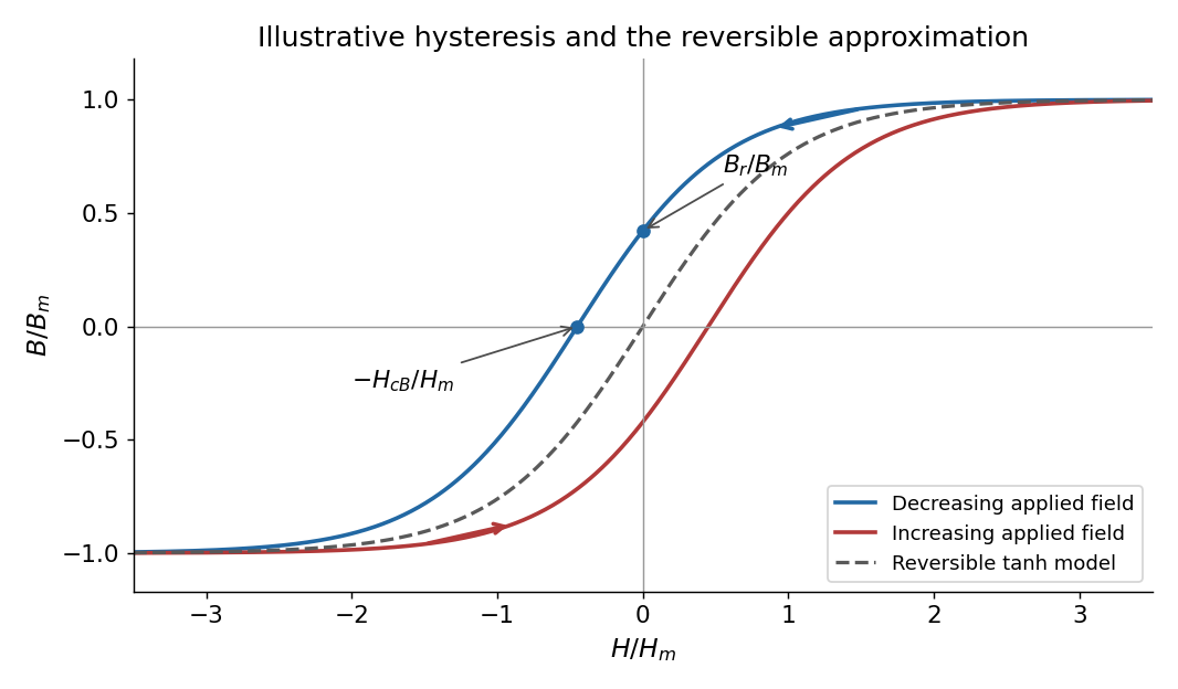
Magnetic hysteresis and the reversible tanh approximation
. Original illustrative magnetic hysteresis loop with the remanent magnetic field and normal coercive magnetic field strength marked. The dashed single-valued curve is the reversible approximation used in the calculation, rather than a hysteresis branch. Details.Use the stated single-valued constitutive equation for the calculation. Inverting it gives , soSince , the small-signal response of a gapped magnetic core isThe small-field core magnetic permeability is . Strictly, is a reversible approximation: at it has , so it cannot itself model nonzero remanence. The displayed loop and this constitutive approximation serve different purposes. Keeping a genuinely remanent branch would generally add a history-dependent offset; it would not imply through the origin.
Take as the centre-to-centre separation and . Use the ideal lossless two-conductor transmission line model, with nonmagnetic surroundings and negligible internal-wire inductance. Opposite line charges and approximate the cylindrical conductors when . Integrating their electric fields, or adding their logarithmic electric potentials, gives the potential differenceThis is the two-wire capacitance at large separation. For opposite electric currents and , the magnetic fields between the wires add. The linked magnetic flux per unit length is approximatelyThus the external inductance of a thin two-wire line is . The lossless telegrapher's equations give a forward wave with , so its characteristic impedance isThe product also gives the propagation speed , an independent consistency check. The exact ideal external-field geometry replaces by . If the wire separation were specified between surfaces, its centre separation would be , with the same leading large-separation result. Finite electrical conductivity and internal-wire magnetic energy require a more detailed line model.
Snell's law is , with both angles measured from the interface normal vector. Let be the meridional ray's angle to the optical axis inside the core and let be the incident medium's refractive index. At the entrance face,At the cylindrical wall the angle of incidence is . For , the critical angle for total internal reflection satisfies . At the limiting accepted ray,Consequently the optical fiber acceptance angle obeysThe requested expression follows for incidence from air, , provided the right-hand side is at most one. Strict total internal reflection occurs inside this limiting cone. The derivation uses the standard meridional ray model; skew launches need additional geometry.
If , every forward entrance angle allowed by this ideal model meets the side-wall condition, and the limiting half-angle is , rather than an undefined inverse sine. For example, , , gives . Thus the unsaturated printed formula is not valid for every possible pair of refractive indices.
Use the thin lens sign convention in which a real object on the incident side has positive object distance, a real image on the outgoing side has positive image distance, and a converging lens has positive focal length. The first image distance isFor the image distance for two separated thin lenses, the second lens has object distance , which can be negative when its intermediate object is virtual. Applying the thin lens equation again givesThe image is beyond the second lens when ; denotes a virtual image on its incident side. A vanishing denominator with nonzero numerator denotes an image at infinity. The rational expression also supplies appropriate limits when the first image is at infinity; for example, gives for finite nonzero focal lengths.
As , the effective focal length is andFor a real incident object, , and positive , the real-image condition is exactly , yielding the requested inequality. This includes two converging lenses. The positivity assumption matters: with and , one has and , but is virtual. If , the touching pair has zero net optical power and produces no real image of this real object in the ideal thin lens model.
Put the plate behind the slit at transverse coordinate , and let positive screen coordinate point toward that slit. The extra optical path length isIn the paraxial approximation, the covered path minus the uncovered path has total optical path difference . Its zero determines the shifted central interference fringe:toward the slit covered by the plate. Moving toward that slit shortens its geometric path and compensates the extra delay in the plate.
More generally, the phase difference is , so every interference fringe translates by the same in this approximation. The spacing is unchanged, and the shift corresponds to fringe periods. For an ideal uniform transparent plate that changes only the wave phase, the envelope and interferometric visibility are unchanged. Reflection losses or unequal transmission through a real plate could additionally reduce the interferometric visibility; those are separate amplitude effects. No numerical wavelength is needed for the physical displacement of the zero-order fringe.
Write and for homogeneous scalar material constants, and use . Taking the curl of Faraday's law of induction and substituting the Ampere-Maxwell law givesThe vector calculus identity for a double curl therefore yieldsThe second term represents electric current response, rather than displacement current. A dispersive is used in the frequency domain; its general time-domain counterpart is a temporal response convolution.
For the convention , the plane wave equation isDecompose the electric field into components parallel and perpendicular to . With , the longitudinal eigenvalue is and each transverse eigenvalue is ; thus the determinant is . For a transverse electromagnetic wave, andwhen and the background . A real dissipative electrical conductivity generally makes complex, with the decaying branch chosen for a passive medium.
For a cold, collisionless, unmagnetized plasma, treat ions as stationary and write for the magnitude of the elementary charge. The electron equation of motion is , soThis reactive response includes no collision-induced Joule heating. Substitution into the transverse dispersion relation givesThe quantity is the electron plasma frequency. The refractive index is real above this cutoff; below it, the wave is evanescent. The electron response is represented here by , so it must not also be counted a second time in the background permittivity.
For a nonzero longitudinal component, taking the dot product of the matrix equation with instead gives . The same cold plasma response makes , henceAt nonzero , the remaining equation forces to be parallel to , and Faraday's law of induction gives . These are electrostatic Langmuir waves, with no dependence of angular frequency in the zero-temperature model. Equilibrium neutrality does not forbid their perturbed charge density; Gauss's law requires such a density when .
Let be the uniform charge density and take . Rigid rotation produces current density . The magnetic dipole moment isSpherical symmetry gives , while . ThereforeIt is parallel to the angular velocity for positive and antiparallel for negative . The fully signed magnitude statement is ; the printed magnitude assumes positive and positive angular speed.
Axisymmetry permits a purely azimuthal magnetic vector potential, , with . For the source's associated Legendre function convention, , since its definition omits the Condon–Shortley phase. The given differential operator reduces toInside the sphere, . Since the radial operator maps to , the particular coefficient is . Regularity at the origin and decay at infinity giveThere is no surface sheet electric current, so both normal and tangential magnetic field components are continuous at . Usingthis is equivalent to continuity of and . The two equations give and . ThusIn the homogeneous expansion, , in their respective interior and exterior regions; all higher angular orders vanish. Indeed, matching the regular and decaying terms with zero source at forces both coefficients to zero. The outside magnetic field is exactly the magnetic dipole field of , not merely its leading far-field approximation. For a positive moment along , , which is the printed cross-product magnitude expression.
For the flux coupling of a rotating charged sphere to a circular loop, take a loop of radius in the equatorial plane and use Stokes theorem on the regular full vector potential, evaluated around the rim. Its linked magnetic flux isWith , the mutual inductance defined using this effective electric current isIntegrating an ideal magnetic dipole field through the entire disk would incorrectly use its singular expression inside the actual sphere; the rim calculation avoids that error.
For the prescribed time dependence, the quasistatic Faraday's law of induction result and the purely resistive loop approximation givePositive loop electric current is defined to produce a positive magnetic dipole moment, so the minus sign is Lenz's law. This assumes negligible retardation and , where is the loop's self-inductance. If that is not negligible, the governing equation is instead ; alone is insufficient for the exact dynamic response.
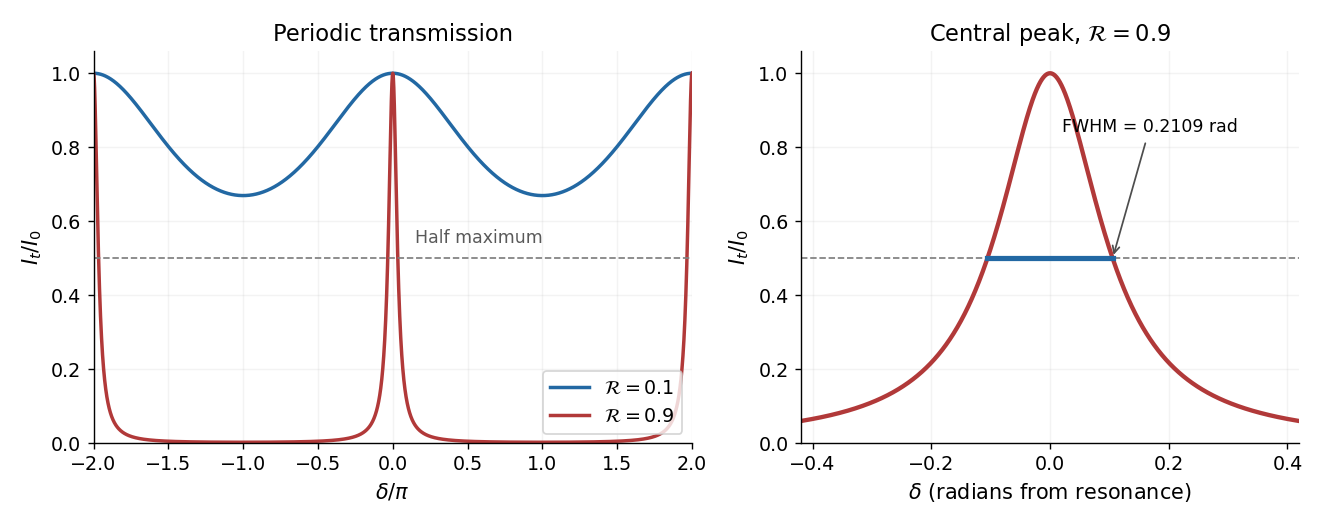
Let be the single-mirror power reflectivity and the propagation angle inside the gas. Define as the vacuum wavelength. Successive transmitted complex amplitudes differ by a round-trip factor , where, for real dielectric reflection coefficients whose product has positive sign,The cosine arises by comparing successive emerging rays on the same outgoing wavefront; it is not the literal zigzag distance . Equivalently, the round-trip phase is . If the source's is the angle in external air, Snell's law gives andIf denotes the internal angle, simply set .
For identical lossless mirrors, their power transmission is . In an energy-normalized amplitude convention this is ; more general interface amplitudes require the corresponding wave impedance factors. The geometric series of transmitted amplitudes givesHenceThis is Fabry–Pérot transmission from multiple reflections.[ref]
Fabry-Perot Interferometer, University of Washington Physics 331. Theory equations (1)–(2), including the coefficient of finesse
At normal incidence, for nondispersive and zero net reflection phase modulo , the resonance condition is . The resonance frequencies and free spectral range areFor finite the resonances have finite width, and transmission away from them is nonzero. Thus “only discrete frequencies” is an ideal high-reflectivity description of the selected resonances, not an exact statement about the support of the transmitted spectrum. For example, at still gives .
At half the unit peak, . Measuring the phase displacement from a resonance yieldsThe last expression is the high-reflectivity approximation, with finesse . At , the full phase width is about radians and . At , the minimum transmission is , so the trace never reaches half the peak and this full width at half maximum is not defined. The exact half-maximum condition requires .
For the absorbing Fabry–Pérot mirror phase and transmission, write and let be the power transmission of one mirror. Optical absorption makes . The transmitted intensity becomesHere the phase formula is at normal incidence. The peak is reduced below unity, while a change in changes the width. The complex reflection phase also moves the resonances: if is approximately constant,If either or depends on frequency, this is an implicit condition and the free spectral range need not be constant. No numerical shift is determined without the mirrors' optical response.
Place the two slits at transverse coordinates and . Let the source point have coordinate and the observation point coordinate , both measured in the same transverse direction. The total lower-slit path minus upper-slit path isThe last line uses the paraxial approximation at both source and screen. The source assumptions give ; the screen expression also assumes . Reversing the source-coordinate orientation would change the sign of , without changing the uniform-source result.
At the slits, the differential path delay from a source element is . Across the full filament its range is . Keeping all these phases nearly equal therefore requiresThis is a sufficient near-unit-spatial coherence condition, rather than a necessary condition for any observable interference. That distinction follows quantitatively below.
Different small elements of a thermal filament are mutually incoherent, so their wave intensities add. The two paths from one element are coherent. If that element supplies the same intensity through each slit, the superposition principle giveswhereIntegrating intensities over the incoherent source givesAdding complex amplitudes across different source elements instead would incorrectly assume mutual optical coherence of the entire filament.
The printed is a signed local modulation, not the usual fringe visibility. From the maximum and minimum of this scanned fringe pattern, the interferometric visibility isIt is independent of the screen's fringe phase and is nonnegative. For a concrete distinction, take and : the printed is zero at that observation point, while the pattern has contrast . The same example has , which is not much smaller than , yet substantial interference survives. When the signed coherence factor is negative, bright and dark fringe positions interchange; the contrast remains its absolute value. This is the distinction between signed coherence and fringe visibility.
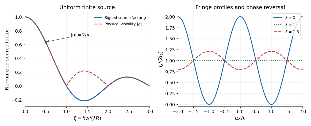
Finite source width changes fringe contrast and can reverse fringe phase
. Original uniform-filament calculation. The signed source factor and its absolute value differ; the latter is the standard interferometric visibility. The fringe traces illustrate high contrast, vanishing contrast, and phase reversal. Details.Source paper: www.whatdotheyknow.com/request/physics_past_exam_papers_2015_16/response/973997/attach/3/Cowell%20Attachment.zip?cookie_passthrough=1 (member: Finals papers/A10431W1_A3_2016.pdf). The dated cover identifies the ordinary Part A sitting of 17 June 2016. All optional questions are included below. Lettered scopes separate successive marked blocks where the source leaves them unlettered.
Insert hydrogen energy eigenstates on either side of the commutator. Because is Hermitian and has eigenvalue ,ThusThis is a necessary electric-dipole selection rule, not a sufficient condition for a nonzero matrix element. For example, by parity even though . The angular factor additionally requires : multiplication of a spherical harmonic by gives only harmonics with the same and adjacent . The commutator alone establishes only the magnetic quantum number restriction; radial integrals and the remaining electric-dipole selection rules for hydrogen must still be considered.
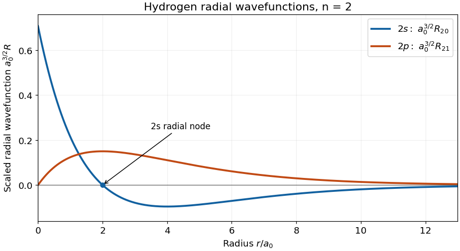
Separation of variables in the central Coulomb potential gives . The radial wavefunction depends on and , independently of . For the hydrogen radial wavefunction in the first excited shell, put . The Bohr radius is , where is the electron–proton reduced mass. Choose the real phasesNear the origin, , whereas . More generally, regular hydrogen radial wavefunctions behave as . At large , both displayed functions have a polynomial factor proportional to multiplying ; approaches zero from below and from above with these phase choices.
The radial wavefunction crosses zero once, at , and has its negative minimum at . The radial wavefunction has no radial node at positive , and reaches its maximum at . The count is ; neither the origin nor the limit at infinity is counted as a radial node. These are sketches of , rather than of or the radial probability density .
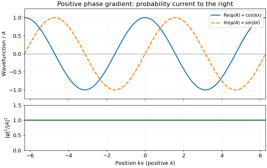
For the Schrödinger equation with a real scalar potential and no vector potential, the probability current isTogether with the probability density , it satisfies the continuity equation . Substituting givesA complex wavefunction requires both its real and imaginary parts in the sketch. Choosing the irrelevant constant phase so that is real, they are and , while the probability density is horizontal. It is the spatial phase gradient of a Schrodinger wavefunction that determines the sign of the probability current. In particular, and have the same real part but opposite probability currents, so the slope of the real part cannot determine the direction.
A nonzero plane wave on the whole real line is not square integrable. The displayed density is understood with box normalization, generalized normalization, or as a local description of a broad wave packet; it does not define a normalized probability distribution on the whole line.
Use the orthonormal energy eigenstates of the infinite square well,The identity resolves the initial wavefunction into . Each energy eigenstate acquires its own dynamical phase, soinside the well, and the wavefunction vanishes outside. The energy probabilities are and at every time. ConsequentlyFor the left half, each diagonal integral is , whileThe interference term therefore yieldsThis probability lies between approximately and , with period . A conserved energy distribution is compatible with time-dependent position probabilities because the relative quantum phase keeps evolving.
Identify the nonrelativistic mass with the rest mass, . Expanding the relativistic kinetic energy in givesFirst-order perturbation theory requires . Put , so . The annihilation relations are and . In particular, does not vanish. A short calculation retaining the operator ordering givesEquivalently, of the ordered words in , only and have nonzero ground-state expectation values, respectively and . Words with a creation operator on the far left or an annihilation operator on the far right vanish; the remaining unbalanced words also vanish. ThusThe correction is negative because the relativistic kinetic energy is smaller than at fixed nonzero momentum. This relativistic oscillator ground-state kinetic correction requires .
For two spin one-half particles, . Squaring givesTake real so that is Hermitian. Since , the displayed polynomial implies . There is a common orthonormal eigenbasis, so all three observables can be simultaneously certain in a common eigenstate. Commutation does not mean that every quantum superposition has definite values of all three.
Suppress the fixed individual quantum numbers . In the coupled basis, ordered on both rows and columns as , the total-spin eigenvalues giveHere the first three entries form the triplet state sector and the last is the singlet state. For the product basis, useThe first term has diagonal entries . Each nonzero exchange term flips to or back, with coefficient . With rows and columns ordered as ,The change of basis is made explicit by and , with . The resulting eigenvalues reproduce the diagonal coupled matrix.
The spin Hilbert space is a tensor product of two two-dimensional spaces and therefore has dimension four. Angular momentum addition decomposes it asThese are three orthogonal triplet states and one singlet state. For identical electrons the complete wavefunction must also satisfy fermionic exchange symmetry: a symmetric triplet spin factor accompanies an antisymmetric spatial factor, whereas the antisymmetric singlet spin factor accompanies a symmetric spatial factor. If both electrons occupy the same spatial orbital, only the singlet spin factor is allowed. The four-dimensional spin space does not assert four allowed spin states for that particular spatial occupation.
Expanding the total angular momentum and replacing transverse components by ladder operators givesThe particle exchange operator obeys and , with the reverse relation for index . These statements also apply to the ladder operators. Exchanging the indices preserves and ; it interchanges the last two terms in . Operators on different tensor factors commute. HenceThe full particle exchange includes the spin coordinates as well as the spatial coordinates.
Write . Each term has cancelling components, so . In the formula for , the first three terms contribute . The two ladder products exchange the two terms and contribute another . ThereforeThis spin state is symmetric; the accompanying spatial state must be antisymmetric for two electrons. A labelled product alone is not an eigenstate of spin exchange: its exchanged vector is orthogonal to it. Thus it cannot supply a definite exchange symmetry when multiplied by a fixed symmetric spatial factor.
This does not prohibit opposite spins in different spatial orbitals. For example, with orthonormal orbitals , the Slater determinantis a valid antisymmetric two-electron state. What fails is treating persistent particle labels as physically distinguishable identities without the required antisymmetrization.
For a conditional spin measurement of identical fermions addressing the component in one spatial mode, the Born rule givesConditioned on this result, the mode spin state is ; the other outcome produces . The spin product is not a spin-exchange eigenstate. The measurement has selected an addressed mode and recorded an outcome, so this conditional spin description distinguishes the measured subsystem.
The full electron wavefunction still obeys fermionic exchange symmetry. For example, the conditional spin-up outcome in spatial mode is represented in particle coordinates byIt is antisymmetric under full particle exchange. Thus the loss of a definite symmetry of the conditional spin product does not mean that measurement turns identical electrons into distinguishable particles. If the outcome is discarded, the mode spin state is instead the equal mixture of the two opposite-spin products. The measurement must specify which spatial mode is addressed for the conditional statement to be operationally meaningful.
Hermiticity of the Cartesian angular momentum components givesThe angular momentum commutation relations implyFor example, . The two terms in cancel in pairs, giving the first commutator. Also .
The spherical harmonics satisfyCommuting or past therefore givesFor a nonzero result these are the eigenvalue equations with unchanged and shifted magnetic quantum number. Taking the squared norm, using , fixes the conventional coefficient:At the appropriate endpoint the coefficient is zero. The zero vector is not itself an eigenstate.
There is no allowed spherical harmonic with , so . The equation first gives . Combining the differential expressions for yieldsIts annihilation of the highest-weight state becomesIntegrating gives , with the constant solution included for . HenceThe phase is single valued for integral orbital quantum number ; normalization fixes only , leaving a conventional constant phase.
Direct integration over solid angle givesThus . Choosing the usual alternating sign convention,Apply successively and divide by its ladder coefficient at each step. Explicitly,The normalization follows because the product of the squared ladder coefficients is . This constructs every magnetic sublevel, including negative .
Separate the center-of-mass motion from the relative motion. Two equal quark masses give reduced mass . Replacing the hydrogen Coulomb strength by gives the Coulomb binding energies and length scaleThe factor of two in the reduced mass matters: using directly would double the binding energy. These are relative binding energies measured from the free quark–antiquark threshold; the rest energy is excluded.
Ignoring spin and working in the fixed quarkonium internal sector, the orbital degeneracy is . HenceNo extra spin or colour multiplicity is being counted. The degeneracy between different at fixed is special to the Coulomb potential.
The linear confinement correction to Coulomb bound states uses , and its first-order energy correction in a normalized Coulomb eigenstate is . Replace by in the hydrogen wavefunctions. The normalized spherical harmonics remove the angular integral, leavingFor , the integral of yieldsFor , put and square the full radial polynomial, including its cross term:For , the same calculation givesConsequently the first two Coulomb levels become, to first order,Thus the second level splits into a singlet orbital level and a triply degenerate orbital level, with . For the confining sign , lies lower than : its smaller mean radius gives the smaller positive correction. The expansion assumes these corrections and the induced couplings to other principal shells are small compared with the relevant Coulomb energy gaps; is the governing small parameter for fixed low .
The unperturbed level is degenerate. The useful point is that a central perturbation is already diagonal within its usual orbital eigenbasis:Angular orthogonality removes the possible mixing of and , and also the mixing of different magnetic sublevels. Therefore the matrix required by degenerate perturbation theory needs no further diagonalization: its diagonal entries are precisely the expectation values above. It would be incorrect to justify the calculation by claiming that the unperturbed spectrum was nondegenerate.
For the energy needs only . For a nonzero central confinement term the energy generally needs , but remains independent of . The magnetic quantum number is still needed to specify an individual orbital eigenstate, rather than just its energy.
With and ,ThusFor , spin down is the lower energy eigenstate. The negative electron magnetic moment is already accounted for in the positive coefficient multiplying in the given Hamiltonian.
In the ordered basis , the transverse magnetic field producesThe off-diagonal complex exponentials follow directly from . This matrix is Hermitian at every time.
Insert the expansion with amplitudes and the two unperturbed dynamical phases into . Differentiation of the explicit phases cancels , leavingEquivalently, with ,These interaction-picture equations conserve . They are exact for the circularly rotating magnetic drive; a rotating-wave approximation has not been used.
Differentiate and substitute the equation for . The result isPutting removes the first derivative and gives , where . For the general solution isThe initial spinor fixes , and the first-order coupled equation fixes the second initial datum . Thus , , andTheir squared magnitudes sum to one. If both and vanish, the initial amplitudes simply remain ; the formulas have that continuous limit.
Source convention correction. For positive , the printed expression for lacks the factor required by the stated basis and initial vector. A concrete test is its derivative at : the printed expression gives , whereas the Schrödinger equation gives . Multiplying only by a phase changes the relative quantum phase. One may change the overall phase of the entire spinor, but must then transform and its initial amplitude as well. The printed modulus nevertheless gives the correct transition probability.
On Rabi resonance, and , soFor nonzero drive the probability starts at zero, reaches unity at , and repeats with period . The population oscillation therefore has angular frequency . This is complete resonant Rabi transfer; a drive of zero strength gives no transition.
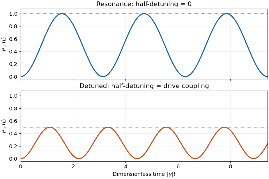
Resonant and detuned spin transition probabilities
. The dimensionless time is the drive coupling times time. The detuned example uses half-detuning equal to the drive coupling, making the maximum transition probability one half. Details.For nonzero Rabi detuning,The sketch starts at zero and oscillates between zero and , with period when the coupling is nonzero. Relative to resonance, the oscillations have a smaller maximum and a shorter period at fixed coupling. The sign of the Rabi detuning changes the amplitudes' phases but leaves this transition probability unchanged. For , its maximum is approximately , so population transfer is strongly suppressed. The plotted detuned example has , giving maximum .
A state function is determined by the equilibrium state, rather than the path used to reach it. Its differential is exact and its change around a closed thermodynamic cycle is zero. Internal energy, entropy and enthalpy are examples; transferred heat and work are not state functions.
For slow expansion in contact with a large thermal reservoir, the fixed temperature of that reservoir maintains an isothermal process. For a fixed amount of ideal gas, internal energy and enthalpy depend only on temperature, soThe ideal gas law also gives . For a reversible expansion the absorbed heat equals the work done by the gas, while its entropy increases by ; constant internal energy does not mean zero heat transfer.
With a thermally insulating boundary, . If the slow piston motion is frictionless and reversible, it is an isentropic process:The first law of thermodynamics gives , so expansion lowers the internal energy and temperature. For constant heat capacity ratio , and are constant combinations of state functions. Insulation alone does not guarantee constant entropy: an irreversible adiabatic process can produce entropy. The conclusion uses the intended reversible, quasistatic piston idealization.
For steady insulated flow through a porous plug, neglect changes of bulk kinetic energy and gravitational potential energy, and allow no shaft work. Each amount of gas brings flow work upstream and delivers downstream. The steady energy conservation balance isThus enthalpy is conserved in this Joule-Thomson effect. For an ideal gas, , so and as well. The entropy increases:The porous-plug process is irreversible despite being slow and insulated; it is not the reversible expansion of the preceding part.
In the one-mole Van der Waals equation, represents excluded volume: the volume available to molecular motion is , rather than . Subtracting in the denominator therefore increases the repulsive contribution to pressure. The term represents intermolecular attraction, which reduces the outward momentum flux at a wall and hence appears as the negative correction . The two minus signs do not mean that both physical effects lower pressure.
For a reversible isothermal process along a homogeneous gas branch with , the work done by the gas isTo find the internal energy change without guessing a caloric law, combine with the Helmholtz free energy Maxwell relation . This givesThereforeThe attractive contribution becomes less negative as the gas expands: separating attracting particles requires energy. This differs from the ideal gas result at fixed temperature. The required heat is . Below the critical temperature, an equilibrium path crossing a liquid–gas coexistence region needs the equilibrium coexistence construction rather than the unstable homogeneous Van der Waals isotherm.
The Clapeyron equation for molar latent heat is . Neglect the liquid molar volume, treat the vapor as an ideal gas, and approximate as constant over the interval. ThenUsing one atmosphere as givesThis is the effective molar enthalpy of vaporization inferred from the Integrated Clausius-Clapeyron relation. If varies with temperature, the inferred value is weighted by , not an unweighted arithmetic mean. Real helium is not exactly an ideal gas over the whole interval, and its liquid changes superfluid state within it, so this is an estimate under the stated approximations rather than a precise temperature-independent material constant.
A magnetic field favors alignment of the magnetic moments of a paramagnet, reducing the number of substantially occupied magnetic configurations at fixed temperature. Its magnetic entropy therefore decreases as the field magnitude increases, explaining the negative sign of .
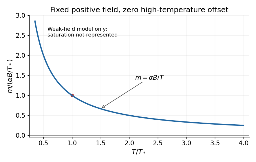
Choose the magnetic Helmholtz free energy convention . Equality of its mixed partial derivatives gives the magnetic Maxwell relationThe magnetic moment inferred from an entropy derivative, integrated at fixed , isThe given entropy derivative alone cannot determine the temperature-independent function . With the usual independent-paramagnet condition as at fixed , , giving Curie's law, . The sketch uses that additional condition. The inverse- expression applies in the weak-field regime; its divergence cannot describe the actual low-temperature saturation of a finite set of magnetic moments.
For reversible quasistatic thermal isolation, . With positive field-dependent heat capacity ,Reducing a positive therefore lowers : this is adiabatic demagnetization. Equivalently, reducing cools for either field sign. Reduced alignment would raise magnetic entropy at fixed ; cooling compensates so total entropy remains constant. Insulation without reversibility would allow additional entropy production and need not follow this adiabat exactly.
Assume a stationary temperature profile, spatially uniform mass density and radioactive heat generation rate, constant thermal conductivity, isotropic solid thermal conduction, and blackbody emission into effectively cold surroundings. The volumetric source isTotal radiogenic power equals the surface blackbody radiation loss. The Stefan–Boltzmann law givesFor steady radiogenic heating of a conducting sphere, the interior heat equation isRegularity at the centre removes the integration term and yields . Matching givesThe high central temperature is compatible with a cold surface because finite thermal conductivity requires a large temperature gradient to carry the accumulated interior heat. A nonzero background radiation temperature replaces by in the surface balance. The calculation neglects convection, stored transient heat, changing radioactive abundances, phase changes and any substantial external irradiation.
Articles were limited to the first 100 out of 110 total.



