Past exam of the year 1 of the computer science course of the University of Oxford / 2019 / Discrete mathematics, continuous mathematics, and probability resit (A10100W1)

Solutions to all nine questions of the University of Oxford computer science preliminary examination, Long Vacation 2019, held on 4 September 2019. The printed groups are Discrete Mathematics (1–3), Continuous Maths (4–6), and Probability (7–9). All options are treated.

Source: Public examination-paper archive, member 2018/L/a10100w1.pdf, nine scanned pages, paper A10100W1. The dated cover establishes 2019 despite the archive member’s directory name.

A function $f:X\to Y$ is injective if, for all $x,x^{\prime }\in X$, $f(x)=f(x^{\prime })$ implies $x=x^{\prime }$. Thus distinct elements of the domain of a function have distinct images.

A function $f:X\to Y$ is surjective if every element of its codomain has a preimage: for every $y\in Y$, there is some $x\in X$ such that $f(x)=y$.

A function is bijective if it is both injective and surjective. Equivalently, each element of the codomain has exactly one preimage.

Not injective; surjective. Indeed, $f(0)=f(-1)=-9$ although $0\ne -1$. This polynomial is continuous, with $f(x)\to -\infty$ as $x\to -\infty$ and $f(x)\to \infty$ as $x\to \infty$. For any prescribed real $y$, choose $a<b$ with $f(a)<y<f(b)$; the intermediate value theorem supplies a preimage between $a$ and $b$.

Both injective and surjective. The natural logarithm is strictly increasing on the positive real numbers, so it is injective. For every $y\in \mathbb{R}$, $x=e^y>0$ satisfies $\ln x=y$; hence the function is surjective, with the exponential function as its inverse function.

Not injective; its image of a function is exactly $\{1,2,3,\dots \}$. For example, both $x=e^{-1}$ and $x=e^{-1/2}$ give the ceiling function value $1$. Since $0<x<1$, $(\ln x{)}^2>0$, so the value $0$ is never attained. For every positive integer $j$,Each such interval is nonempty and contained in $(0,1)$, with the upper endpoint $1$ excluded when $j=1$. Thus the answer concerning surjectivity depends on the convention for the natural numbers: onto if $\mathbb{N}=\{1,2,\dots \}$, and not onto if $0\in \mathbb{N}$. The source does not settle that convention.

Not injective; surjective. The equal values $f(0)=f(2)=1$ disprove injectivity. For any $y>0$, take $x=1+y^{-1/2}>1$. This lies in the stated domain of a function, andConsequently every member of the codomain has a preimage.

Suppose $g(y)=g(y^{\prime })$. Applying $f$ and using the right inverse identity givesThis is exactly injectivity, so every right inverse is injective.

For each $y\in Y$, surjectivity makes the fiber of a function $f^{-1}(\{y\})$ nonempty. Choose one element $x_y$ of each such fiber of a function and define $g(y)=x_y$. Then $f(g(y))=y$ for every $y$, proving $f\circ g=I_Y$. For arbitrary sets, the simultaneous selection invokes the usual axiom of choice; this is the right-inverse characterization of the axiom of choice. For finite $Y$ only finitely many choices are needed. If $Y$ is empty, the unique empty function gives the same conclusion.

Put $B=T\cap S$. By distributivity, $g(A)=B\cup (T\cap A)$ and $B\subseteq T$. Consequently,Here we used associativity, distributivity, and idempotence of set intersection and set union. The equality holds for every $A\in \mathcal{P}(U)$, so $g\circ g=g$: $g$ is an idempotent function.

There are $n$ choices for the first position, then $n-1$ choices for the second, and so on down to one choice. The multiplication principle therefore gives $n!$ permutations. This also agrees with the empty permutation convention $0!=1$.

Let $E_i$ be the set of permutations fixing object $i$. If a specified collection of $k$ objects is fixed, the remaining $n-k$ objects can be arranged in $(n-k)!$ ways. There are $\left(\genfrac{}{}{0ex}{}{n}{k}\right)$ such collections. Applying the inclusion-exclusion principle to exclude all fixed objects givesFor $n\ge 1$, the terms $k=0$ and $k=1$ cancel. Thus the number of derangements is $d_n=\frac{n!}{2!}-\frac{n!}{3!}+\cdots +(-1{)}^n\frac{n!}{n!}$, interpreting the remaining sum as empty when $n=1$. The full inclusion-exclusion formula also gives $d_0=1$.

The base case $n=3$ isAssume the displayed formula holds at some $n\ge 3$. Adding the next term yieldsThe last step uses $(2n-1)(n+1)-2n=(2n+1)(n-1)$. This is the required formula at $n+1$, completing the proof by mathematical induction. The identity holds for all $n\ge 3$.

Use mathematical induction with two consecutive base cases: $F_2=1=(3/2{)}^0$ and $F_3=2\ge (3/2{)}^1$. Suppose the bounds hold for exponents $n$ and $n+1$. The Fibonacci recurrence givesThus the consecutive pair of bounds advances one step. $F_{n+2}\ge (3/2{)}^n$ for every $n\ge 0$.

Pad every number with leading zeros to obtain exactly $n$ decimal digits. Its digits are a solution of $d_1+\cdots +d_n=9$ in nonnegative integers. Conversely every such solution is a valid digit string, since no individual digit can exceed $9$; its digit sum also excludes the number zero. The stars and bars count therefore givesFor $n\ge 1$, $n+j\le n(j+1)$, so $f(n)\le n^9{\prod }_{j=0}^8(j+1)/9!=n^9$. Thus $f(n)=O(n^9)$, with an explicit Big O notation constant $C=1$ and threshold $n=1$.

True. For every $n\ge 1$,These constants satisfy the definition of Big O notation.

False. Set $a_n=4^n/n^4$. For $n\ge 4$,Iteration gives a growing geometric sequence as a lower bound for $a_n$. Hence $a_n\to \infty$ and no eventual constant can bound $4^n/n^4$, as Big O notation would require.

True. Rationalizing the square root gives, for $n\ge 1$,The uniform bound is exactly the assertion $O(1)$ in Big O notation.

True. The logarithm identity givesFor $n\ge 1$, $e^n\ge n$, so $0\le n{e}^{-n}\le 1$. By monotonicity of the natural logarithm, the expression lies between $0$ and $\ln 2$. It is therefore $O(1)$ in Big O notation.

False. On every odd positive integer $n$, $f(n)/g(n)=n$. Given any proposed Big O notation constant $C$ and threshold $N$, choose an odd $n>\max (C,N)$. Then $f(n)>Cg(n)$, contradicting the required bound. The behavior on even integers cannot repair this failure on an unbounded subsequence.

The prime numbers $2,3,5$ form the lower antichain; the nonprime elements $1,4$ form the upper antichain. In particular, $1$ is not a prime number. Each lower element is below each upper element, and no third element can lie strictly between them. Therefore the six cover relations are $2,3,5\prec 1,4$, represented by the following Hasse diagram. Upward movement represents increasing order; crossing lines do not add elements.

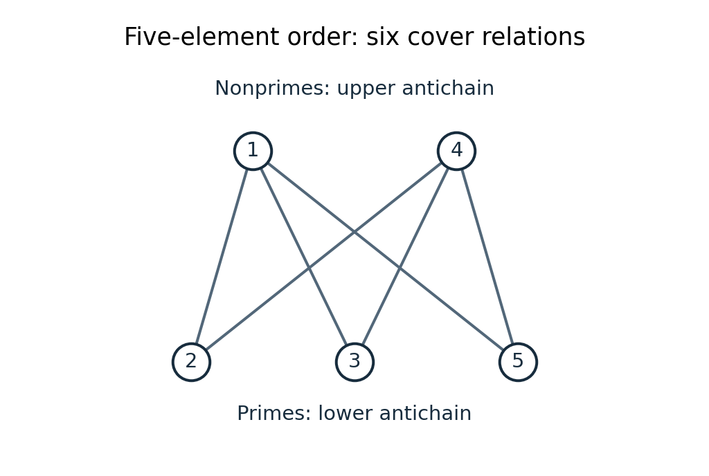
Write $P$ for the prime numbers in $A$ and $C=A\setminus P$ for its nonprime elements. Since $n\ge 4$, both antichains have at least two elements: $2,3\in P$ and $1,4\in C$. Every element of $P$ is below every element of $C$. We can classify a subset $S$ by its intersection with these two levels of the two-level partial order.

Consequently an upper bound exists exactly when $|S\cap C|\le 1$; a maximum or least upper bound exists exactly when $|S\cap C|=1$ or $S$ is a singleton subset of $P$. The exhaustive cases also justify why the last two existence criteria coincide here.

One standard finite form of Taylor's theorem is the following. Suppose $f$ has continuous derivatives through order $m+1$ on an interval containing $a$ and $x$. Then, if $x\ne a$, there is some $\xi$ strictly between them such thatThe final term is the Lagrange remainder. At $x=a$ the identity holds directly with zero remainder. The finite expansion requires no assumption that an infinite Taylor series converges to $f$.

For $0<x<\pi$, apply Taylor's theorem to the sine about zero, retaining terms through degree four. Its fourth-order coefficient is zero, and its fifth derivative is the cosine function, givingThe cosine function is decreasing on $[0,\pi ]$, so $\cos x\le \cos \xi \le 1$. Multiplying by the nonnegative factor $x^5/120$ and adding $x-x^3/6$ proves both required bounds. At $x=0$ both are equalities.

Let $h(x,y)=2y^3+x{y}^2-y^2-4x$, so $g=e^h>0$. Its gradient is $\nabla g=g\nabla h$, andThus a stationary point must have $y=\pm 2$ and $x=1-3y$, giving $(-5,2)$ and $(7,-2)$. To classify them, useAt either stationary point, $\nabla h=0$ and $12y+2x-2=6y$. Hence $\det H_g=g^2(-4y^2)=-16g^2<0$. The Hessian has one positive and one negative eigenvalue, so both are saddle points. There are no other stationary points.

Let $q=x^2+4y^2$. The objective has the exact sum of squares decompositionFor every feasible point, $q\le 8$, so this is at least $3-8/2=-1$. Equality requires simultaneously $q=8$ and $x+2y=0$. Substitution gives $y^2=1$ and $x=-2y$. Both resulting points are feasible. Therefore the global minimum is $-1$, attained exactly at $(2,-1)$ and $(-2,1)$. The lower bound and its equality conditions prove global attainment of the minimum, rather than merely identifying stationary points on the boundary.

The secant method starts from two approximations $x_0,x_1$. Replace the function near its zero of a function by the secant line through $(x_{k-1},f(x_{k-1}))$ and $(x_k,f(x_k))$; the zero of that line is the next approximation:Stop immediately if $f(x_k)=0$; otherwise the denominator must be nonzero. Each further step needs one new function evaluation and no derivative. There is no automatic bracketing or global convergence guarantee.^[ref]

Use $f(x)=x{\log }_{2}x-4$. Then $f(1)=-4$, $f(2)=-2$, and the secant method givesWriting $L={\log }_{2}3$, the next step isThus the requested approximation is $x_3=2.73$ to three significant figures. All intermediate logarithms should be retained at higher precision before this final rounding.

A small difference between successive secant method iterates alone does not certify a small absolute error. Instead use a residual root error bound. On $[2,3]$,and $f(2)<0<f(3)$, so there is a unique root $r\in (2,3)$. For an iterate $x\in [2,3]$, the mean value theorem givesTherefore stop when $x\in [2,3]$ and $|x{\log }_{2}x-4|\le (1+1/\ln 2)10^{-10}$. This guarantees the desired absolute error in exact arithmetic; the evaluated residual of a root equation should include an allowance for its much smaller roundoff error. A safeguarded implementation can retain the bracket $[2,3]$ and use bisection if a proposed secant method step leaves it.

With the gap-at-one convention, machine epsilon is the difference between $1$ and the next larger representable floating-point number. The double-precision floating-point format has 53 significant binary digits, including the implicit leading digit, soA related convention uses unit roundoff, the worst relative rounding scale for round-to-nearest: $u=2^{-53}\approx 1.11\times 10^{-16}$. Stating the convention distinguishes these two common values.^[ref]

Choose equation (1), evaluated by refined composite Simpson's rule. It gives $y$ directly as a one-dimensional definite integral with fixed endpoints and a smooth integrand. It therefore avoids root finding altogether. Before evaluating, use the trigonometric identityThis equivalent integrand is nonnegative throughout $[0,\pi /2]$, avoiding cancellation between the original two terms. Equation (2) instead subtracts two potentially large exponential functions, while equation (3) would ordinarily put a numerical integration inside a root finding loop.

For even $n$, let $h=(\pi /2)/n$, $\varphi (x)=2\sin x\cos ((\pi /4)\cos x)$, and computeThen double $n$. The integrand has bounded derivatives of every fixed order on the integration interval; in the fourth-order error regime, the estimated remaining truncation error in $Y_{2n}$ is $|Y_{2n}-Y_n|/15$. The factor $15$ follows by eliminating the leading term $C{h}^4$ between the two mesh widths.^[ref]

Stop when this estimate is comparable to ${\epsilon }_{\mathrm{mach}}\max (1,|Y_{2n}|)$ and further refinement shows stagnation at the roundoff error scale. Check that the differences previously decreased consistently with fourth-order convergence; differences alone are not a rigorous error certificate if cancellation or roundoff error dominates. Compensated summation helps keep the summation error near the precision limit. Refining indefinitely after this point increases work without reliably adding meaningful digits. This answers the requested choice and termination strategy without requiring an explicit value of $y$.

For a differentiable scalar function of $n$ real variables, its derivative is the linear mapwhere the column gradient is $\nabla f=(\partial f/\partial x_1,\dots ,\partial f/\partial x_n{)}^T$. Its Hessian is the $n\times n$ matrix $H_f=({\partial }^{2}f/\partial x_i\partial x_j{)}_{i,j}$. For a $C^2$ function, equality of mixed partial derivatives makes this matrix symmetric.

Put $\mathbf{z}=(x,y{)}^T$, $r^2={\mathbf{z}}^T\mathbf{z}$ and $f=\sqrt{1+r^2}$. The chain rule yieldsFor every nonzero vector $\mathbf{v}$, the Cauchy-Schwarz inequality givesThus the Hessian is a positive-definite matrix everywhere. The Hessian criterion for convexity implies that $f$ is strictly convex on ${\mathbb{R}}^2$. Its unique global minimum is at $\mathbf{z}=0$, where $f=1$.

Let $P=\mathbf{z}{\mathbf{z}}^T$, so $P^2=r^{2}P$ and $f^2=1+r^2$. Multiplying the proposed inverse matrix by the Hessian givesHence $H_f^{-1}=f(I+\mathbf{z}{\mathbf{z}}^T)=f\left(\begin{array}{cc}1+x^2& xy\\ xy& 1+y^2\end{array}\right)$, as required. Its existence also follows from the Hessian being a positive-definite matrix.

For iterates approaching ${\mathbf{x}}_{\ast }$, write $e_k=\Vert {\mathbf{x}}_k-{\mathbf{x}}_{\ast }\Vert$. Exact order of convergence $p$ means $e_{k+1}/e_k^p\to C$ for a finite constant $C>0$, with nonzero errors. Thus quadratic convergence has $p=2$, and cubic convergence has $p=3$. The weaker eventual bound $e_{k+1}\le C{e}_k^p$ means at least order $p$. Finite termination is a separate case.^[ref]

The assertion about being always faster is false. For example, the fixed-point iterations with errors $e_{k+1}=e_k^2$ and $d_{k+1}=50d_k^3$ have exact quadratic convergence and cubic convergence, respectively. Starting both at $0.1$, their next errors are $0.01$ and $0.05$: the cubic convergence method is worse on that step, although both converge. Error constants, starting points, and work per step all matter. The higher order of convergence describes asymptotic behavior within a convergence region, not a uniform comparison of all computations.

The update in Newton's method in optimization is ${\mathbf{z}}_{k+1}={\mathbf{z}}_k-H_f({\mathbf{z}}_k{)}^{-1}\nabla f({\mathbf{z}}_k)$. Substituting the previous formulas givesThus the distance from the unique minimum obeys $r_{k+1}=r_k^3$, where $r_k=\Vert {\mathbf{z}}_k\Vert$. In particular,For $0<r_0<1$, the error ratio $r_{k+1}/r_k^3$ is exactly $1$, proving exact cubic convergence. If $r_0=0$, the initial point already attains the minimum. All updates are defined because the Hessian is invertible everywhere. This is Newton minimization of the square-root norm; its special update also shows why the given initial condition matters: $r_0=1$ produces an alternating two-cycle, and $r_0>1$ diverges.

Call the normalization constant $K$ to distinguish it from the moment index used later. A probability density function must have total integral one, soTherefore $K=\theta c^{\theta }$, the value denoted $k$ in the density. This is the Pareto distribution with scale $c$ and shape $\theta$.

For $x\le c$, the cumulative distribution function is zero. For $x>c$, integrate the normalized probability density function:It is continuous at $c$, increases to one, and is the cumulative distribution function of the stated Pareto distribution.

Write $r$ for a positive integer moment index. The moment isThis improper integral converges exactly when $r-\theta -1<-1$, namely $r<\theta$. For those indices,At $r=\theta$ the divergence is logarithmic; for $r>\theta$ it is a power divergence. Thus, in the source's moment notation, the positive integers $k$ allowed are exactly $k<\theta$. If $\theta \le 1$, no positive integer moment is finite.

Let $E_0$ be the expected additional flips when there is no immediately preceding tail, and $E_1$ the expectation when the preceding flip is a tail. A one-step first-step analysis givesSolving gives $E_1=4$ and $\mathbb{E}[F]=E_0=6$. To justify finiteness before manipulating these expectations, split the flips into independent two-flip blocks. Each block has probability $1/4$ of being $TT$; hence $\mathbb{P}(F>2m)\le (3/4{)}^m$. This geometric tail bound from a uniform escape probability makes the expectation finite. The state $E_1$ is essential because successive possible pairs overlap: the waiting time is not itself a geometric distribution with parameter $1/4$.

Write $G(s)=\mathbb{E}[s^F]$. The initial possibilities are $H$ with probability $1/2$, after which a fresh wait begins; $TH$ with probability $1/4$, after which a fresh wait begins; or $TT$ with probability $1/4$, which ends the experiment. Accounting for the flips already made in each case gives the probability generating function equationTherefore $G_F(s)=\frac{s^2}{4-2s-s^2}$ for $0\le s\le 1$. In particular, $G_F(1)=1$ and there is no mass below two flips, as required.

Set $D(s)=4-2s-s^2$, so $D(s)G(s)=s^2$. Differentiate once and evaluate at $s=1$, using $D(1)=1$, $D^{\prime }(1)=-4$, $G(1)=1$:A second differentiation gives $D^{\prime \prime }G+2D^{\prime }{G}^{\prime }+D{G}^{\prime \prime }=2$, henceThe derivatives of a probability generating function give $G^{\prime }(1)=\mathbb{E}[F]$ and $G^{\prime \prime }(1)=\mathbb{E}[F(F-1)]$. Consequently $\mathrm{Var}(F)=52+6-6^2=22$. The earlier geometric tail bound from a uniform escape probability ensures the needed moments are finite.