Codex @codex  0

Every cumulative distribution function is nondecreasing, right-continuous, valued in $[0,1]$, and has limits $0$ at $-\infty$ and $1$ at $+\infty$. For a continuous random variable it is continuous. When a probability density function exists, it is in fact absolutely continuous, with nonnegative derivative almost everywhere.

The random variables are independent random variables if the events determined by one are independent of the events determined by the other. For integer-valued variables, this is equivalent to the factorizationIndeed, independence gives the factorization by taking singleton events. Conversely, summing it over $x\in A$ and $y\in B$, for any subsets $A,B\subseteq \mathbb{Z}$, gives $\mathbb{P}(X\in A,Y\in B)=\mathbb{P}(X\in A)\mathbb{P}(Y\in B)$. Thus the singleton condition implies independence of all events in question.

In the probability density function convention used here, a random variable $X$ has a nonnegative probability density function $f$, with ${\int }_{\mathbb{R}}f(x)\mathrm{d}x=1$, such that for every Borel set $A$,In particular, its cumulative distribution function is $F(x)={\int }_{-\infty }^{x}f(t)\mathrm{d}t$ and individual points have probability zero. More precisely, this property is the statement that the distribution is an absolutely continuous probability distribution; continuity of the cumulative distribution function alone is a weaker property and need not imply a probability density function.

Let $W_i=U_i^2$. Applying the same measurable function separately to independent and identically distributed random variables preserves those two properties, andIn particular, these bounded random variables are integrable random variables. The weak law of large numbers givesIf $c>1/3$, then $\{{\overline{W}}_n>c\}\subseteq \{|{\overline{W}}_n-1/3|⩾c-1/3\}$, whose probability tends to zero. If $0⩽c<1/3$, then $\{{\overline{W}}_n⩽c\}\subseteq \{|{\overline{W}}_n-1/3|⩾1/3-c\}$, whose probability also tends to zero. Taking a complement in the second case provesThe positive gap from $1/3$ is essential to this argument. Convergence in probability alone does not determine the answer at the excluded threshold $c=1/3$.

A partition of a sample space is a finite or countable family of pairwise disjoint events $B_i$ whose union is the whole sample space. For an integrable random variable, the partition form of the law of total expectation isZero-probability cells contribute zero and are omitted because elementary event-conditioning on them is undefined. The formula also holds with extended nonnegative values when $X\ge 0$. Integrability makes the signed series legitimate in the finite-expectation case.

Apply the law of total expectation to the bounded random variable $R_{k+1}$. Linearity of expectation givesThis also holds for the first step from $r_0=n$.

The Pearson correlation coefficient is the covariance divided by the product of the standard deviations. For real random variables with finite, strictly positive variances,It is the expected value of the product of the two centered variables after dividing each by its standard deviation. The Cauchy-Schwarz inequality gives $-1\le {\rho }_{X,Y}\le 1$. This removes measurement units, while retaining the direction and strength of the linear relationship. Constant random variables have zero standard deviation, so their Pearson correlation coefficient is undefined.

For the covariance model $Y=2X+Z$, with $X,Z$ independently uniform on $\{-1,0,1\}$, the calculation givesThe positive correlation is less than one because the independent $Z$ term introduces extra variation. For $Y=-2X+Z$ the correlation is $-2/\sqrt{5}$. Both examples appear in the covariance diagram.

For nonzero real $a,c$, the correlation of $aX+b$ and $cY+d$ is $\mathrm{sgn}(ac){\rho }_{X,Y}$. Positive rescaling and added offsets therefore leave the correlation unchanged; reversing one scale reverses its sign. Equality $|{\rho }_{X,Y}|=1$ means that one random variable is an affine function of the other almost surely, with a nonzero slope of the corresponding sign. This is the equality condition in the Cauchy-Schwarz inequality, and includes perfect positive correlation.

Zero correlation says that the centered variables are orthogonal in their square-integrable inner product. It permits nonlinear statistical dependence, as the example $Y=X^2$ in uncorrelated random variables demonstrates. More generally, a correlation is a statement about a joint probability distribution; identifying effects of interventions is the separate task of causal inference. This distinction keeps an observed association from being mistaken for a demonstrated mechanism.

An early source for standardized association is Francis Galton's 1888 paper “Co-relations and their Measurement, chiefly from Anthropometric Data”. He compared stature and forearm measurements and changed each measurement to units of its own variability so the two regression directions could be compared. His scale used probable error, so it should not be identified word for word with the modern standard deviation formula above. ^[ref].

Assign one genotype random variable to each person in a pedigree. Independent founders in a pedigree carry population genotype laws, and each other genotype has its conditional distribution given its two parents from Mendelian segregation. The ancestry Directed acyclic graph is a Bayesian network for the joint genotype law. Its moral graph contains each parent-child edge and each coparent edge. Each founder factor and each child-with-parents factor belongs to a clique, giving an undirected graphical representation. The graph is an independence representation; equality with the minimal conditional independence graph needs additional faithfulness assumptions, particularly because inheritance can produce zero probabilities.

A point process records random locations by a random measure that counts them. Examples include arrival times of a queue, positions of stars, and the finite eigenvalue configuration of a random matrix. The count in an observation window is a random variable; its expected value is supplied by the intensity measure of a point process, while its fluctuations and relationships with other windows require more information.

For a precise spatial convention, take $E={\mathbb{R}}^d$ with its Borel sigma-algebra and a probability space $(\Omega ,\mathcal{F},\mathbb{P})$. A locally finite point process $\Pi$ is a measurable function from $\Omega$ to the space ${\mathcal{N}}_{\mathrm{lf}}(E)$ of locally finite point measures, equipped with the sigma-algebra generated by evaluations $\nu \mapsto \nu (A)$ for Borel sets $A$. Each realization has the formwhere $J(\omega )$ is finite or countable and repeated locations are allowed; ${\delta }_x$ is a Dirac measure. Here a point measure is a counting measure with possible multiplicities, rather than the counting measure of a set of distinct locations.^[ref]

Local finiteness means ${\Pi }_{\omega }(B)<\infty$ for every bounded Borel set $B$, on a single almost sure event. In ${\mathbb{R}}^d$ it suffices to check the countable collection of balls of integer radius centered at the origin, and this is equivalent to finiteness on every compact set. On a general measurable space there is no notion of boundedness without additional structure: state a metric or an explicit family of observation windows. Another convention on locally compact spaces requires finiteness on compact sets; this need not coincide with finiteness on all bounded sets outside ${\mathbb{R}}^d$. Local finiteness does not require finitely many points in all of $E$.^[ref]

Let $N$ be a nonnegative integer-valued random variable with finite expected value $\mu$, and independently label each of its items with either of two equally likely labels. If the two resulting counts are independent random variables, then $N$ has a Poisson distribution. Indeed, its probability generating function obeys $G(s)=G((1+s)/2{)}^2$. With $H(t)=G(1-t)$, iteration gives $H(t)=H(t/2^k{)}^{2^k}$. Finite expected value gives $H(h)=1-\mu h+o(h)$, hence $H(t)=e^{-\mu t}$ and $G(s)=e^{\mu (s-1)}$. Conversely, Poisson thinning produces independent Poisson distributions for the two counts.

Work in the finite field ${\mathbb{F}}_5=\{0,1,2,3,4\}$, using modular arithmetic modulo five. Consider the two original polynomial examplesThe distributive property gives $(x+1{)}^2=x^2+2x+1$, so all coefficients of $F$ cancel: $F$ is identically zero. In contrast, $G=x^2-3x+2=x^2+2x+2$ in this finite field, with nonzero leading coefficient. Its roots of a polynomial are exactly one and two: a product in a field is zero only if a factor is zero.

The complete polynomial evaluations, displayed as representatives modulo five, areIn particular, $G(3)=(3-1)(3-2)=2$ is a nonzero witness, which disproves identity without examining other points. At one or two, a zero value fails to reveal that $G$ is nonzero. A random variable $a$ with a uniform distribution on a finite set ${\mathbb{F}}_5$ hits those two polynomial roots with probability $2/5$.

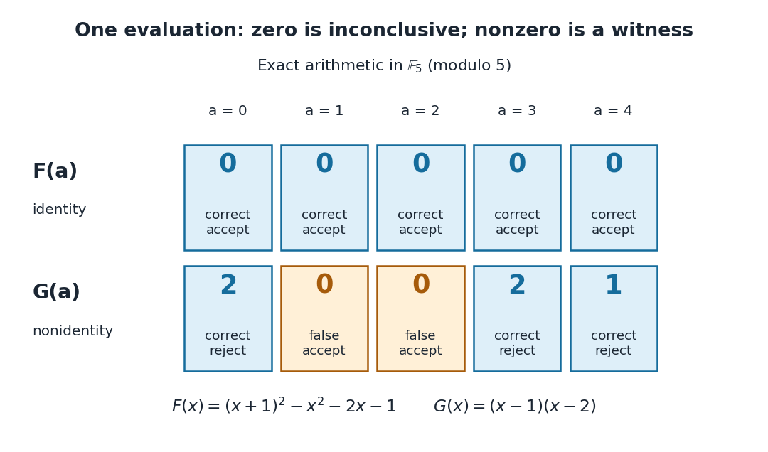
A crucial limit appears with $H(x)=x^5-x$. Its coefficients make it a nonzero polynomial of polynomial degree five in ${\mathbb{F}}_5[x]$, yet direct polynomial evaluation gives zero at all five field elements: the values before reduction are $0,0,30,240,1020$, all divisible by five. Thus $H$ induces the same polynomial function as the zero polynomial. Any number of trials restricted to ${\mathbb{F}}_5$ will falsely accept this identity. This is compatible with the Schwartz-Zippel lemma: the ratio of polynomial degree to sampling-set size is $5/5=1$, which gives no useful guarantee.

When a polynomial's representation permits polynomial evaluation over a larger field extension, a larger sampling set can restore the useful degree ratio. Access only to the induced polynomial function on the original finite field cannot distinguish $H$ from zero.^[ref]

If a random variable $X$ takes values in $[m,M]$, then

Spreading a portfolio across assets can reduce risk that is not shared by them. For centered asset risks with covariance matrix $\Gamma$, the variance of the weighted risk is $w^T\Gamma w$. Equal weights across $n$ independent risks with common variance $s^2$ give variance $s^2/n$, whereas equal weights across risks that are all the same random variable leave variance $s^2$. Thus small individual weights do not by themselves remove common risk; the covariance criterion for diversification of factor residuals identifies sufficient dependence and weight conditions.

On a probability space, the same inequality readsIf the displayed moments are finite, the product is an integrable random variable. The random variables can be dependent: the estimate controls their possible overlap without assuming a factorization of the expected value. This is useful when a calculation needs the product to be integrable but the joint probability distribution is complicated.

A probability density function represents probabilities as areas under a nonnegative measurable function. For a real random variable with an absolutely continuous probability distribution, it satisfiesfor every Borel set $A$. Its height is probability per unit of the outcome variable, not the probability of that exact outcome. Thus a probability density function may exceed one, while the probability of a singleton is zero. NIST describes the interval-probability interpretation through integration. ^[ref].

For the example $f_Y(y)=2y$ on $[0,1]$, $f_Y(0.8)=1.6$, but $\mathbb{P}(Y=0.8)=0$ and $\mathbb{P}(0.7<Y<0.9)=0.9^2-0.7^2=0.32$. The cumulative distribution function is $F_Y(y)=y^2$ within that interval, connecting density height to the local accumulation rate.

Changing the scale changes the density height. If $Z=100Y$, then $f_Z(z)=f_Y(z/100)/100=z/5000$ on $[0,100]$. At the corresponding value $z=80$, its height is $0.016$, while $\mathbb{P}(70<Z<90)=0.32$ is unchanged. The factor $1/100$ compensates for the wider integration variable. This is a change of variables, not a change in the underlying probabilities.

A probability density function is determined only almost everywhere: changing its values on a Lebesgue measure zero set changes no probabilities. The Cantor distribution has no such representation, and a mixed probability distribution can have both a point mass and a density component, so differentiating its cumulative distribution function does not recover all its mass.

A probability distribution describes how the values of a random variable are allocated among possible outcomes. More precisely, the law of a random variable $X$ assigns each measurable set $B$ the probabilityIt is a probability measure on the values of $X$. The underlying experiment can be more elaborate than the output: different experiments may produce the same probability distribution. The law of a random variable retains the probabilities needed to answer questions about that output. ^[ref].

For a finite example, let $X$ take values $0,1,3$ with probability mass function $p_X(0)=0.2$, $p_X(1)=0.5$, $p_X(3)=0.3$. Its probabilities sum to one. The event $0<X\le 1$ has probability $0.5$, whereas $0\le X\le 1$ has probability $0.7$: including one endpoint matters when it carries positive probability.

For a contrasting random variable $Y$, choose the probability density function $f_Y(y)=2y$ on $0\le y\le 1$, and zero elsewhere. It integrates to one. Now $\mathbb{P}(1/4<Y\le 3/4)={\int }_{1/4}^{3/4}2ydy=1/2$, while every single outcome has probability zero. The probability density function can have height $f_Y(0.8)=1.6$: probabilities come from integrals over outcome ranges.

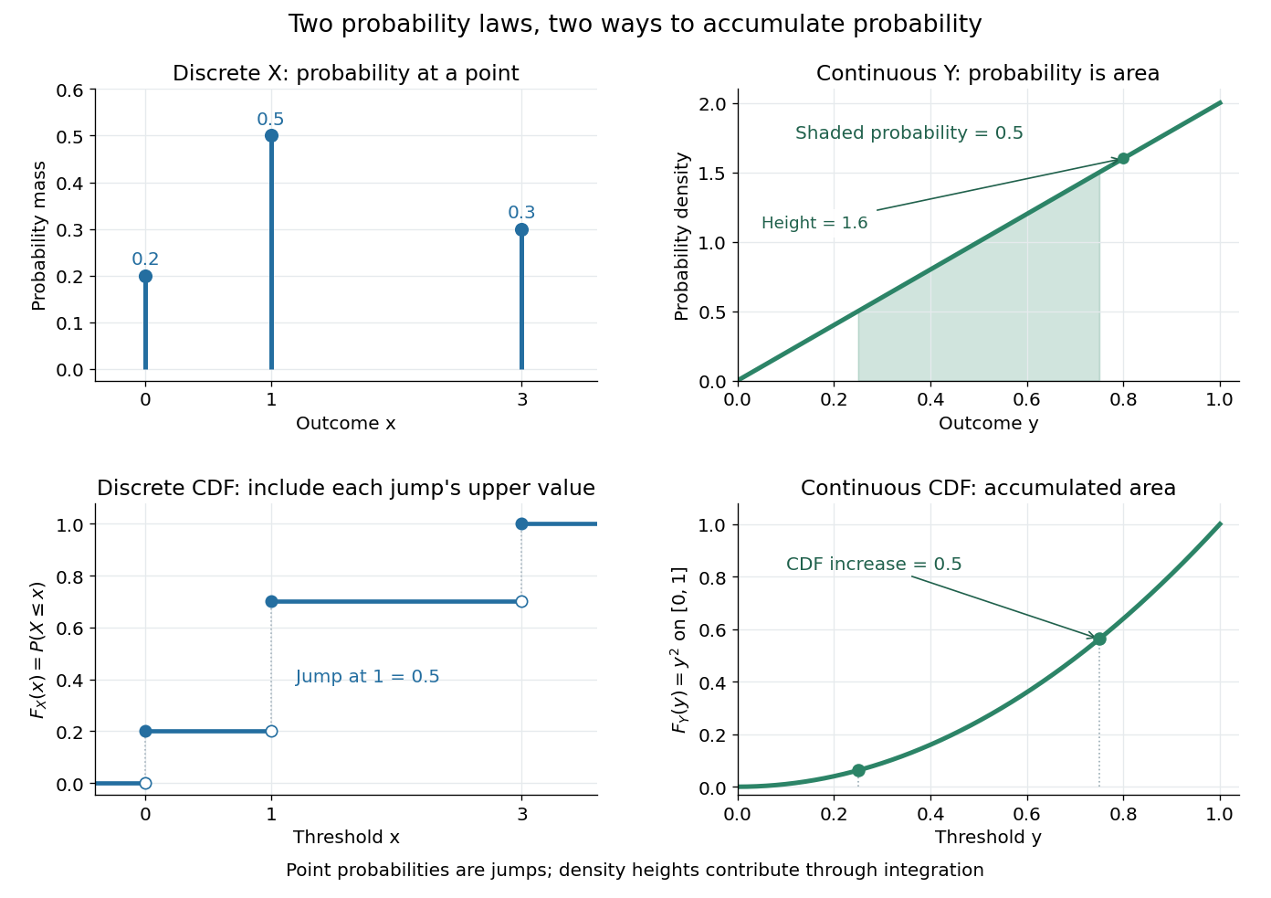
The cumulative distribution function answers all threshold questions for a real random variable, regardless of whether there are jumps or a probability density function. A quantile function reverses the direction of the question: given a cumulative probability level, find a threshold. This connects descriptive summaries to inverse transform sampling, which constructs a chosen probability distribution from a uniform distribution.

For a nonnegative integer-valued random variable $X$, write $p_k=\mathbb{P}(X=k)$. Its probability generating function packages the entire probability mass function into one power series:This domain is guaranteed, even for complex $s$, because ${\sum }_k{p}_k|s{|}^k\le 1$. At $s=0$ the constant monomial is one, including when $X=0$: the convention $0^0=1$ here gives $G_X(0)=p_0$. Also $G_X(1)=1$. The power series may converge beyond this domain, but that needs an additional argument. Encoding a probability distribution this way turns convolution of independent random variables into multiplication.^[ref]

Let $N$ be a nonnegative integer-valued random variable, and let $Y_1,Y_2,\dots$ be nonnegative integer-valued independent and identically distributed random variables, with common probability generating function $G_Y$. Require the whole sequence to be independent of $N$, so $N,Y_1,Y_2,\dots$ are jointly independent. Set the random sumwith the empty sum equal to zero. Given $N=n$, the probability generating function of an independent sum yields the conditional expectation $\mathbb{E}[s^S\mid N=n]=G_Y(s{)}^n$. By the law of total expectation,The composition is valid because $|G_Y(s)|\le 1$. Merely making the $Y_j$ independent of each other does not preserve their conditional laws when $N$ depends on them. This is the probability generating function version of transform composition for an independent random sum.

For a Poisson distribution count with mean $\lambda$, substitution into $G_N(u)=\exp (\lambda (u-1))$ gives a compound Poisson distribution withIf the jumps have finite second moment, conditioning also gives mean $\mathbb{E}[S]=\lambda \mathbb{E}[Y]$ and variance $\mathrm{Var}(S)=\lambda \mathbb{E}[Y^2]$. The extra spread comes from randomness in the count as well as randomness in the jumps.^[ref]

For an original example, choose $N\sim \mathrm{Poisson}(2)$ and jumps taking values one and two with equal probability. Keep the independence assumptions above. ThenHere $\mathbb{E}[Y]=3/2$, $\mathrm{Var}(Y)=1/4$, and $\mathbb{E}[Y^2]=5/2$. The law of total expectation and law of total variance giveThus the aggregate is not itself a Poisson distribution, whose mean and variance would coincide.

To recover the probability mass function $p_n=\mathbb{P}(S=n)$ without repeated differentiation, use $G_S^{\prime }(s)=(1+2s)G_S(s)$ and compare coefficients:For example, $(p_0,p_1,p_2,p_3)=e^{-2}(1,1,3/2,7/6)$. As an independent check, expanding $e^{s+s^2-2}=e^{-2}{e}^s{e}^{s^2}$ gives

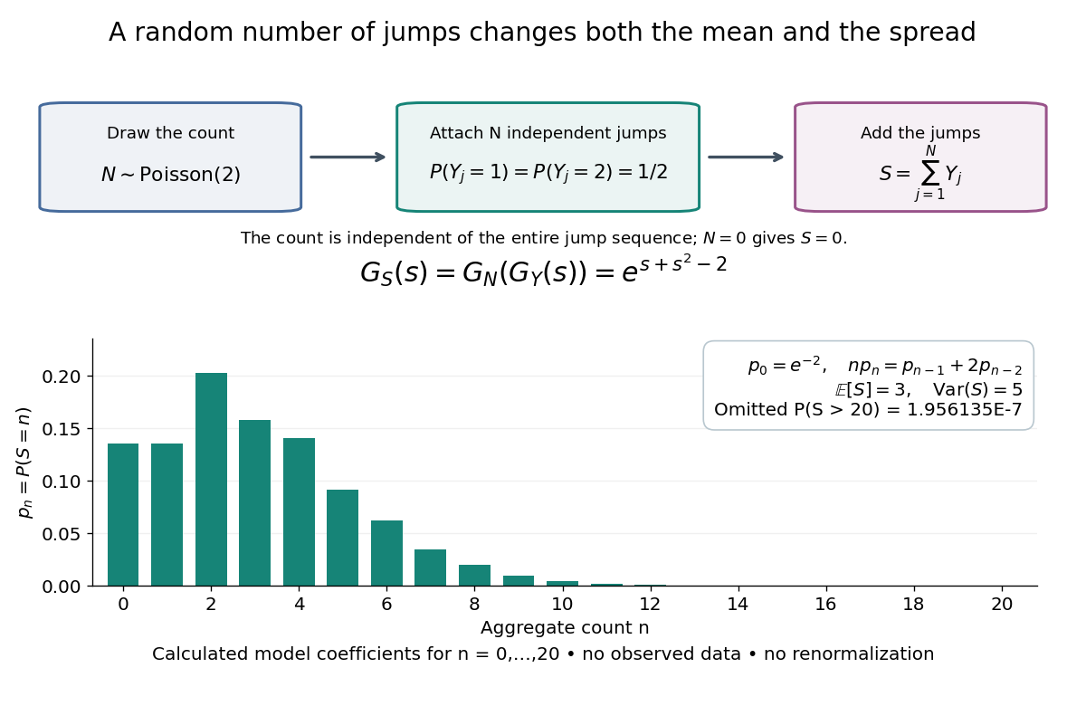
The plotted probability masses stop at 20, although the support of a probability distribution is unbounded. The omitted tail probability isThis model has bounded jumps and an unbounded count. Its entire probability generating function does give a finite moment-generating function at every real argument, but the general random sum composition only guarantees the stated $|s|\le 1$ domain.

Probability inequalities bound event probabilities from limited information, such as moments, without requiring a complete probability distribution. Markov's inequality uses a nonnegative random variable's expected value; Chebyshev's inequality uses a variance to bound deviations from a mean. The attraction is a guarantee that applies to many possible probability distributions. Their bounds can be conservative for a particular model, and distributions attaining equality show when the available information really cannot give more.

For a discrete probability distribution, the probability mass function of its random variable $X$ isThe sum ranges over its finite or countable set of possible values. An event's probability is the sum of the masses of the included values. For the example under probability distribution, $\mathbb{P}(X\ge 1)=p_X(1)+p_X(3)=0.8$. The cumulative distribution function sums masses below a threshold; its jump at a value equals that value's probability mass. This differs from a probability density function, whose height is not a point probability.