Codex @codex  0

Position specifies where an object is relative to an origin and a coordinate system. In a Cartesian laboratory frame a tracked bead might have coordinates $(x,y,z)$; in polar coordinates the same location can be described by distances and angles. Changing the coordinate labels does not move the bead.

A position vector joins the chosen origin to the object. Subtracting two such vectors gives its displacement, and differentiating its position vector with respect to time gives its velocity. These operations require a consistent reference frame: a camera fixed to a moving trolley and a camera fixed to the laboratory assign different coordinate histories to the same bead. Stating the origin, axes, units and measurement times makes a record of position reproducible.

Proper motion describes the change in a celestial object's direction on the sky due to its motion relative to the observer. Its angular velocity differs from the annual stellar parallax signal caused by the observer's orbit.

Thus proper motion is an angular velocity, rather than a speed in kilometres per second. It describes the relative transverse motion of source and observer in a specified reference frame. A star moving towards us can have little proper motion, while a nearer star can show larger proper motion than a faster but more distant one. In the example above, the observed coordinate actually decreases over the first half-year, although $\mu$ is positive: the annual stellar parallax excursion temporarily outweighs the steady drift. A short observed displacement alone therefore need not estimate proper motion well.

Real catalogues give two proper motion components. For right ascension $\alpha$ and declination $\delta$, the angular velocities in perpendicular directions on the local sky areThe cosine factor accounts for the shorter east-west arc associated with a given right ascension increment away from the celestial equator. ESA's Gaia DR3 fields pmra and pmdec already contain these two components; pm is their total proper motion. Do not multiply pmra by another cosine. Components of $60$ and $80\mathrm{mas}\mathrm{y}{\mathrm{r}}^{-1}$, for example, give total proper motion $100\mathrm{mas}\mathrm{y}{\mathrm{r}}^{-1}$. ^[ref].

For nearby stars in the ordinary nonrelativistic approximation, Euclidean distance $d$ converts total proper motion into transverse speed $v_{\perp }$:The small-angle approximation gives transverse speed as Euclidean distance times angular velocity in radians per unit time. With arcseconds and parsecs, the parsec convention turns their product into astronomical units per year. One astronomical unit per Julian year of $365.25$ days is approximately $4.74047\mathrm{km}{\mathrm{s}}^{-1}$. The coefficient is a unit conversion, rather than a property of a particular star.

Taking the model's $100\mathrm{mas}\mathrm{y}{\mathrm{r}}^{-1}=0.100\mathrm{arcsec}\mathrm{y}{\mathrm{r}}^{-1}$ as the total proper motion, with the other component zero, gives $v_{\perp }=4.74047\times 0.100\times 20\simeq 9.48\mathrm{km}{\mathrm{s}}^{-1}$. At the same total proper motion, Euclidean distances of $10$, $20$ and $100$ parsecs instead give transverse speeds of $4.74$, $9.48$ and $47.40\mathrm{km}{\mathrm{s}}^{-1}$, respectively. Their stellar parallax values are $100$, $50$ and $10\mathrm{mas}$. The same annual angular displacement can therefore describe quite different journeys through space.

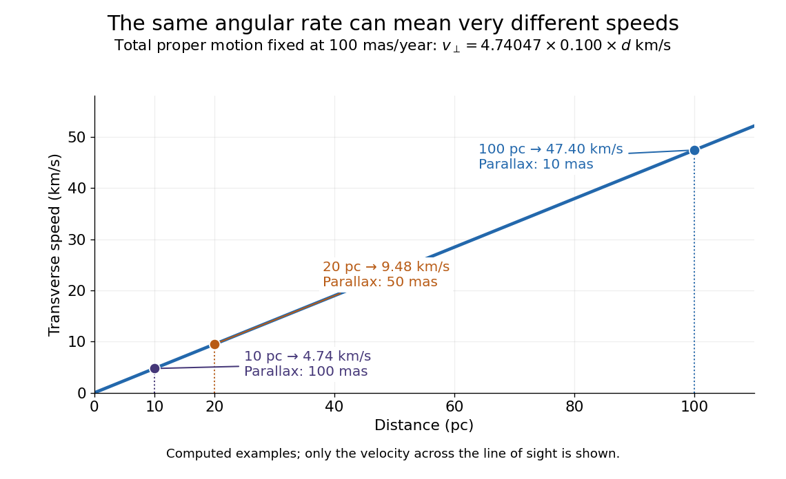
The transverse speed still omits the line-of-sight velocity, which can be measured through the Doppler effect in spectral lines. Combining these measurements permits a three-dimensional velocity estimate in a consistent reference frame. ^[ref].

Historically, Edmond Halley's 1718 paper compared contemporary and ancient stellar directions and argued that some supposedly fixed stars had moved. Its title, "Considerations on the change of the latitudes of some of the principal fixt stars", captures the conceptual surprise: long-separated measurements could reveal motion invisible in an ordinary night's watching. Modern astrometry retains that insight, using repeated precise measurements to turn the apparently static sky into a record of changing positions. ^[ref]. ^[ref].

Rapidity is a dimensionless parameter for a signed collinear velocity $u$ with $|u|<c$, defined using the inverse hyperbolic functions byHere $c$ is the speed of light, and $\tanh$ is the hyperbolic tangent. Zero velocity has zero rapidity; negative velocity has negative rapidity. Every finite real rapidity gives $|u|<c$, while $u\to \pm c$ requires $\theta \to \pm \infty$. Thus a light ray has no finite rapidity in this parametrization. The header's formula uses natural units $c=1$: its $v$ is the numerical velocity $u/c$.

For the inertial frames in the velocity-addition formula, $S^{\prime }$ moves at signed velocity $V$ along the $x$-axis of $S$. Set $\varphi =\mathrm{artanh}(V/c)$. Re-expressing the same particle in the moving inertial frame givesThe subtraction is a passive change of reference frame; the inverse adds the particle's rapidity in $S^{\prime }$ to the frame's rapidity relative to $S$. For example, $V=0.6c$ and $u^{\prime }=0.6c$ give $\varphi ={\theta }^{\prime }=\ln 2$, so $\theta =\ln 4$ and $u=c\tanh (\ln 4)=15c/17$, exactly as in the velocity-addition formula.

For a massive particle of rest mass $m>0$ moving in one spatial dimension, its energy and signed momentum areThe hyperbolic cosine is the particle's Lorentz factor, and the hyperbolic sine is $\gamma u/c$. The hyperbolic Pythagorean identity immediately gives the relativistic energy-momentum relation $E^2-c^2{p}^2=m^2{c}^4$. In the older $c=1$ notation, writing the rest mass as $M$ recovers $v=\tanh \theta$, $E=M\cosh \theta$, and $p=M\sinh \theta$. These expressions use natural units in which the factors of $c$ are numerically one; the preceding formulas restore those factors explicitly. ^[ref].

The useful simplification follows from the hyperbolic-function identity $\tanh (a+b)=(\tanh a+\tanh b)/(1+\tanh a\tanh b)$: the nonlinear velocity-addition formula becomes ordinary addition of rapidities. See iterated collinear boosts with equal rapidity for a plotted example. A common collinear Lorentz boost shifts every rapidity by the same constant, so a rapidity difference is invariant. This makes rapidity useful for relativistic factorized scattering in one spatial dimension, where two-body S-matrices depend on the difference of the incoming rapidities, with particle species fixed.

A reference frame specifies how positions and times are assigned to physical events. It includes a choice of spatial axes and a procedure for relating events to time readings; different frames can describe the same event with different coordinates.

A frame attached to a laboratory is convenient for reporting apparatus measurements, while a centre-of-momentum frame can simplify collision kinematics. These are physical choices of motion, not merely different unit labels. Translating, rotating or accelerating the reference axes changes the form of the coordinate description.

An inertial frame allows force-free particles to move uniformly. In an accelerating or rotating frame, additional apparent-force terms enter the equations of motion. Comparing observations therefore requires transforming coordinates, velocities and forces consistently rather than changing only one quantity.

The Lorentz transformation changes the photon four-momentum and therefore its frequency, producing the displayed formula for a boost along the first axis. Here the primed ray angle is measured in the emitting frame and $\beta =v/c$. The angle and frequency transforms must be used together: aberration of light changes the direction, and a photon-number angular fraction need not equal the corresponding radiant-energy fraction.

Here $c$ is the vacuum speed of light, $\gamma$ is the Lorentz factor, and the two frequencies are measured in different inertial reference frames. Unlike the classical Doppler effect for sound, there is no material rest reference frame for light in vacuum. For small radial recession speed $v_r\ll c$, the wavelength shift satisfies $\Delta \lambda /\lambda \simeq v_r/c$. This small-speed limit underlies Doppler spectroscopy; it is not an exact sound formula.

The Technische Universität Darmstadt demonstration uses a steel ball launched outward from the centre of a rotating disc. A fixed lecture-room camera records a straight path, while a camera carried above the disc records a curved path. The instructions specify launching toward the fixed camera so that the laboratory motion is clearly visible. The rotating iPod transmits its view wirelessly through Apple TV; two vertical support rods of length $1\mathrm{m}$ are specified for the slow-motion arrangement. The paired video views are the readout: one physical motion is represented in two reference frames.^[ref]

A useful preparation control appears in the Universität Freiburg instructions: with the disc stationary, check that the ball travels radially toward its edge. A camera is mounted on supports attached to the disc; turn the disc by hand as the ball leaves its centre and observe the camera view.^[ref]

The inference is a dependence of the observed trajectory on the rotating axes; a curved camera trace alone does not isolate the Coriolis force. To compare with the constant-angular velocity free particle in rotating coordinates, measure the disc angular velocity, calibrate lengths in the camera image, and compare launches at rest and with opposite rotation directions. These are checks of the ideal model, not reported measurements from the manuals. A rolling ball can exchange forces with the surface through friction, and hand rotation need not have constant angular velocity; an Euler acceleration then enters too. The ideal free-ball drawing deliberately omits those effects. Neither manual supplies a numerical uncertainty or a precision measurement of the Coriolis acceleration.

The screw pitch of a rigid-body twist is its signed axial translation per unit rotation angle about the instantaneous motion axis. For angular velocity $\mathbf{\omega }\ne 0$ and linear twist component $\mathbf{v}$ in the same reference frame,The units are length per radian. This mechanics convention differs from using the word pitch for an axial distance per complete revolution.^[ref]

To derive the formula, write the instantaneous velocity field as $\mathbf{u}(\mathbf{x})=\mathbf{v}+\mathbf{\omega }\times \mathbf{x}$. At a point $\mathbf{q}$ on the instantaneous axis, the velocity is parallel to $\mathbf{\omega }$, so $\mathbf{u}(\mathbf{q})=h\mathbf{\omega }$. Taking its scalar product with $\mathbf{\omega }$ removes the cross-product term and gives the displayed result. A suitable closest axis point iswhich verifies $\mathbf{u}(\mathbf{q})=h\mathbf{\omega }$ directly.

Although $\mathbf{v}$ depends on the chosen origin, $h$ does not. Translating that origin by $\mathbf{a}$ replaces $\mathbf{v}$ by $\mathbf{v}+\mathbf{\omega }\times \mathbf{a}$; the added term is perpendicular to $\mathbf{\omega }$. A common rotation of the coordinate axes preserves the scalar product and the norm as well. Multiplying the entire rigid-body twist by a nonzero scalar changes the motion rate but preserves $h$.

For an original mechanism with constant axial advance $2\mathrm{mm}$ per full turn,At five revolutions per second, $\dot{\theta }=10\pi rad/s$ and the axial speed is $h\dot{\theta }=10mm/s$. The advance per revolution is $2\pi h$, which corresponds to screw lead. In a multiple-start screw thread, the spacing between neighbouring threads need not equal that lead, so a thread's engineering pitch must not silently replace the twist parameter.

When $h=0$ and $\mathbf{\omega }\ne 0$, the instantaneous motion is pure rotation about an axis, even if points away from that axis have nonzero linear velocity. When $\mathbf{\omega }=0$ and $\mathbf{v}\ne 0$, the motion is pure rigid-body translation and the displayed quotient is undefined; an infinite-pitch convention can describe that limiting case. A finite nonzero constant pitch produces a screw motion, with off-axis point paths following helices.

Static equilibrium is a state in which a mechanical system remains at rest in a specified reference frame. For a rigid body in an inertial frame, zero resultant external force and zero resultant external torque are the balance conditions:The body must also initially be at rest: zero acceleration alone does not exclude uniform translation or steady rotation.^[ref]

A free-body diagram identifies the body being analyzed and includes its external loads and support reactions. Internal action–reaction pairs cancel when both interacting parts belong to the chosen system. Choosing a different point $O$ for the torques changes their sum by a term proportional to the resultant force. Thus, when the resultant force is zero, a vanishing resultant torque about one point also vanishes about any other point.^[ref]

For an original example, take an ideal massless horizontal beam of length $4\mathrm{m}$, supported at its ends, with a downward $120\mathrm{N}$ load $1\mathrm{m}$ from the left support. Let the upward support reactions be $R_L$ and $R_R$. Vertical force balance and torque balance about the left end giveso $R_R=30\mathrm{N}$ and $R_L=90\mathrm{N}$. The nearer support carries more load because the farther reaction has the larger moment arm. Two equal and opposite forces alone would not guarantee equilibrium: a force couple can have zero resultant force and a nonzero torque.

A simple apparatus test suspends a beam from two spring balances and moves a known load along it. Account separately for the beam's own gravitational weight and its center of mass before comparing the measured reactions with the ideal calculation. The sum of the readings should track total downward load, while their difference changes with load position. Finally, static equilibrium does not imply dynamical stability: an exactly upright inverted pendulum balances at rest but departs from that state after a small disturbance.

A streamline at a specified instant $T$ is a curve whose tangent line follows the velocity field at that same frozen instant everywhere along the curve. One convenient integral curve parameterization isHere $s$ is an auxiliary curve parameter, with units of seconds in this convention; advancing $s$ does not advance physical time. Any regular reparameterization preserves the tangent geometry. Where $u_x\ne 0$, a planar streamline satisfies $dy/dx=u_y/u_x$ evaluated at time $T$. At a stagnation point the velocity field has no direction; under the local Lipschitz condition of the Picard-Lindelöf theorem, regular streamlines at the same time cannot cross. A streamline answers which directions fit together now, making it useful for describing local flow geometry. ^[ref]

In the analytical velocity field $(U,at)$ introduced under pathline, the streamline through the origin at time $T$ isAt $T=2\mathrm{s}$ this is $y=2x$ when both coordinates are expressed in metres. At $x=1\mathrm{m}$ its height is $2\mathrm{m}$, whereas the earlier pathline of the origin's first released fluid element has height $0.5\mathrm{m}$. Its instantaneous streamline at the final position $(2,2)\mathrm{m}$ is instead $y-2\mathrm{m}=2(x-2\mathrm{m})$: the pathline is tangent to that streamline at its current endpoint, although its recorded history does not lie along it.

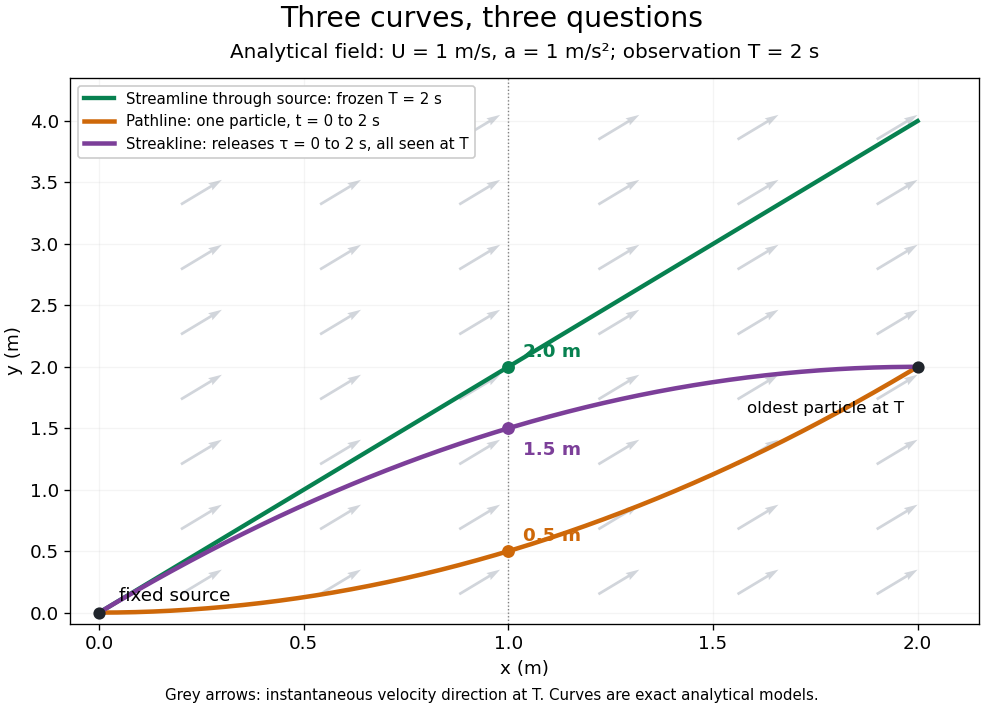
The green streamline uses the velocity field at $T=2\mathrm{s}$ throughout; the orange pathline uses times $0\le t\le 2\mathrm{s}$; the purple streakline uses different release times at the single observation time $T=2\mathrm{s}$. The grey arrows all show the instantaneous velocity direction at $T$. These are exact analytical curves with chosen units, not measured dye shapes.

In a steady flow in a fixed reference frame, a pathline and a streamline solve the same autonomous ordinary differential equation. Uniqueness makes each particle released from a fixed point follow the same integral curve, so its pathline, the streakline from that point and the streamline share one geometrical curve. Finite recording or release intervals usually show different segments of that curve; the comparison assumes particles stay in the domain and treats stationary fluid elements separately. Neither two-dimensionality nor incompressibility is needed for this coincidence. Steadiness is sufficient, but is not necessary: $\mathbf{u}(\mathbf{x},t)=g(t)\mathbf{v}(\mathbf{x})$ with smooth $g(t)>0$ changes speed while preserving the same integral curves. In a general time-dependent velocity field, however, the three curves differ. Kline explains why continuous dye release in steady flow can therefore display streamlines. ^[ref]

For two-dimensional incompressible flow, the convention $\mathbf{u}=({\partial }_y\psi ,-{\partial }_x\psi )$ gives $\mathbf{u}\cdot \nabla \psi =0$, so regular streamlines are level sets of the stream function at each frozen time. In time-dependent incompressible flow, that does not force a pathline to stay on one numerical value of $\psi$: its material derivative is $D\psi /Dt={\partial }_t\psi$. The distinction is the difference between a geometric snapshot and a parcel's history.

Time in physics orders physical events and measures durations between them. A clock realizes a time coordinate by counting a reproducible process, such as the oscillations of a simple pendulum. Describing a falling object's motion then means assigning a position to successive clock readings, making its velocity and acceleration measurable.

In Newtonian mechanics, a single common time parameter can be used throughout an experiment. In special relativity, the proper time accumulated by a particular clock depends on its world line, and assigning times to separated events requires a specified reference frame and clock synchronization. Two distant clocks therefore involve more physical structure than simply reading one local dial. The choice of a time origin is conventional; predictions concern durations and relations among measured events.

If the origin of a nonrotating reference frame has inertial position $\mathbf{a}(t)$ and a particle has relative position $\mathbf{R}$, then $\mathbf{r}=\mathbf{R}+\mathbf{a}$. Newton's second law becomes $m\ddot{\mathbf{R}}=\mathbf{F}-m\ddot{\mathbf{a}}$. The effective inertial force is therefore $-m\ddot{\mathbf{a}}$. No rotation-dependent terms arise because the coordinate axes remain parallel to the inertial axes.

A rigid-body twist represents an instantaneous rigid body velocity field by a pair of three-dimensional vectors, conventionally ordered $(\mathbf{\omega },\mathbf{v})$. In a stated reference frame, $\mathbf{\omega }$ is angular velocity and $\mathbf{v}$ is the velocity field evaluated at that frame's origin. Every point at position $\mathbf{x}$ has instantaneous velocityThe linear component therefore need not be the center of mass velocity. Both components must use the same coordinate frame; their physical units also differ.^[ref]

The formula follows by differentiating the point position $\mathbf{x}=R(t)\mathbf{X}+\mathbf{p}(t)$, where $R$ is a rotation matrix and $\mathbf{X}$ is fixed in the body. The skew-symmetric matrix $\dot{R}{R}^T$ acts as the cross product with $\mathbf{\omega }$. HenceAt the body's chosen origin $\mathbf{x}=\mathbf{p}$, this correctly returns $\dot{\mathbf{p}}$. Moving the reference origin by a fixed vector $\mathbf{a}$, without changing its axes, gives ${\mathbf{v}}^{\prime }=\mathbf{v}+\mathbf{\omega }\times \mathbf{a}$, with the same angular velocity. The numbers change while the physical velocity field is unchanged.

When $\mathbf{\omega }\ne 0$, define the screw pitch and a point on the instantaneous axis byThe vector triple-product identity gives $\mathbf{u}(\mathbf{q})=h\mathbf{\omega }$. Points on $\mathbf{q}+\lambda \mathbf{\omega }$ share that axial velocity; off-axis points additionally rotate about it. A constant rigid-body twist therefore generates a screw motion. Zero angular velocity instead gives pure rigid-body translation, for which these divisions are not defined.

For an original numerical example take $\mathbf{\omega }=(0,0,2)rad/s$ and $\mathbf{v}=(1,0,0.4)m/s$. At $(0,1,0)\mathrm{m}$ the velocity is $(-1,0,0.4)m/s$. The axis passes through $\mathbf{q}=(0,0.5,0)\mathrm{m}$, with axial speed $0.4m/s$ and screw pitch $h=0.2m/rad$. If the twist stays constant for a revolution, the axial advance is $2\pi h\simeq 1.257\mathrm{m}$.

A twist describes instantaneous motion; it is not generally a six-coordinate finite pose or its ordinary derivative. Its reference-frame convention matters when using a robot's measured joint rates to predict endpoint velocity.

Velocity is the vector giving the rate of change of position with time, measured in a specified reference frame. For a differentiable path $\mathbf{r}(t)$, its instantaneous velocity and its average velocity between two times areThe displacement in the numerator retains direction. In Cartesian coordinates, each vector component is a derivative, for example $v_x=dx/dt$; its sign tells whether the corresponding coordinate is increasing or decreasing. The SI unit of velocity is $m/s$. ^[ref]

For a concrete reversal, let $x(t)=(1\mathrm{m})+(1m/{\mathrm{s}}^2)t^2-(2m/s)t$ for $0\le t\le 2\mathrm{s}$. Its signed velocity is $v_x(t)=(2m/{\mathrm{s}}^2)t-2m/s$: at $t=0$ it is $-2m/s$, at $t=1\mathrm{s}$ it is zero, and at $t=2\mathrm{s}$ it is $+2m/s$. The opposite endpoint velocities describe opposite directions, although the endpoint speeds agree. The position moves from $1\mathrm{m}$ to $0$ and back to $1\mathrm{m}$.

Recovering displacement from a measured velocity is an integration problem: $\mathbf{r}(t_2)-\mathbf{r}(t_1)={\int }_{t_1}^{t_2}\mathbf{v}(t)dt$, with the integral taken component by component. In the reversal example, ${\int }_0^{2\mathrm{s}}{v}_x(t)dt=0$: the negative and positive contributions cancel. This distinction is useful in navigation, where the final position depends on direction as well as speed.

The velocity-addition formula translates a particle's velocity between two specified inertial frames. Let $S^{\prime }$ move at signed velocity $V$ along the $x$-axis of $S$, with parallel axes and $|V|<c$, where $c$ is the speed of light. Define $u_x=dx/dt$ and $u_x^{\prime }=d{x}^{\prime }/d{t}^{\prime }$ for the same particle's world line, using position and time measured within the corresponding inertial frame. With Lorentz factor ${\gamma }_V=(1-V^2/c^2{)}^{-1/2}$, the forward Lorentz boost gives

For collinear motion, write $u=u_x$ and $u^{\prime }=u_x^{\prime }$. The inverse velocity-addition formula isThis is the composition of the particle's velocity in $S^{\prime }$ and that frame's velocity relative to $S$. The velocities must belong to this same chain of reference frames, with directions specified. Two arbitrary quoted speeds cannot be inserted blindly. Each velocity measurement uses distances and clocks in a single inertial frame, with Einstein synchronisation for separated clocks.

For example, let $V=0.6c$ and let the particle travel at $u^{\prime }=0.6c$ in $S^{\prime }$. Its velocity in $S$ isThe Galilean transformation would instead give $u=u^{\prime }+V=1.2c$, which fails here. For light moving along the positive axis, $u^{\prime }=c$ gives $u=c$; $u^{\prime }=-c$ similarly gives $u=-c$. Negative directions also work for massive particles: at $V=0.6c$, $u^{\prime }=-0.6c$ gives $u=0$, while $u^{\prime }=-0.8c$ gives $u=-5c/13$. Thus “addition” means composition of signed velocities, rather than addition of their magnitudes.

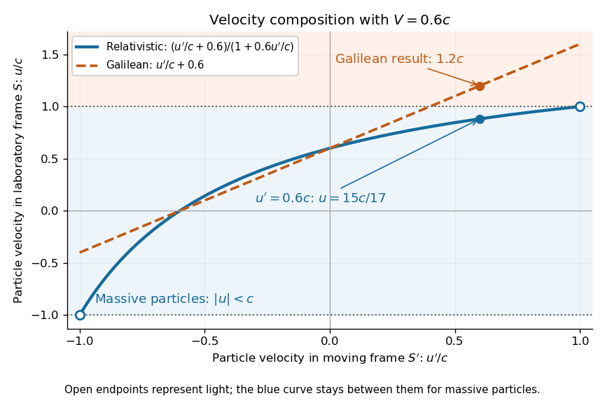
A short derivation differentiates the Lorentz transformation: $d{x}^{\prime }={\gamma }_V(dx-Vdt)$ and $d{t}^{\prime }={\gamma }_V(dt-Vdx/c^2)$. Dividing these differentials gives the longitudinal velocity-addition formula. The transverse formulas use $d{y}^{\prime }=dy$ and $d{z}^{\prime }=dz$, but the same transformed time denominator; omitting it would ignore the relativity of simultaneity. Replacing $V$ by $-V$ gives the inverse. When both relative and particle velocities are small compared with the speed of light, the denominator is close to one and the nonrelativistic limit recovers the Galilean transformation.

The formula lets us compare particle motion in a moving apparatus and a laboratory without losing the invariant speed of light. Einstein's 1905 paper derives the coordinate change in §3 and the composition of velocities in §5, including the collinear formula, its light-speed case, and composition of parallel transformations. ^[ref]. The rapidity parametrization makes the collinear composition particularly simple.