Codex @codex  0

Consider an original model at fixed vacuum wavelength $600\mathrm{nm}$ and temperature $20^{\circ }\mathrm{C}$. Stipulate a transparent sample with Verdet constant $V=20\mathrm{rad}{\mathrm{T}}^{-1}{\mathrm{m}}^{-1}$, length $L=0.050\mathrm{m}$, uniform adjustable $B_z$, and a field-independent analyzer-zero offset ${\theta }_0=0.020\mathrm{rad}$. These are chosen values, not measured glass properties. On a continuously tracked small-angle branch,Taking half the difference gives ${\theta }_{\mathrm{odd}}=0.100\mathrm{rad}$; half the sum recovers ${\theta }_0=0.020\mathrm{rad}$. Hence $V={\theta }_{\mathrm{odd}}/(LB)=20\mathrm{rad}{\mathrm{T}}^{-1}{\mathrm{m}}^{-1}$. A field-reversal difference of $0.200\mathrm{rad}$ is twice the single-field rotation, not that rotation itself. More generally this subtraction removes every contribution that is even under $B\mapsto -B$, provided the sample and apparatus remain otherwise matched.

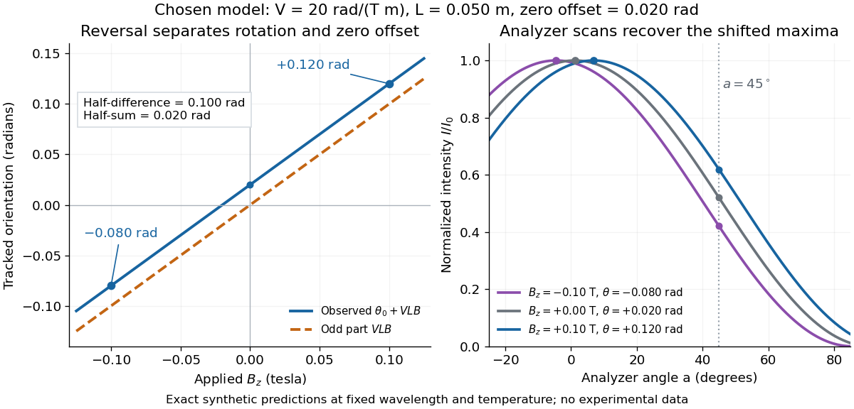
An ideal polarimeter analyzer at laboratory angle $a$ reads normalized light intensity $I(a,B)/I_0={\cos }^2[a-{\theta }_{\mathrm{obs}}(B)]$. Here $I_0$ is the light intensity immediately before the analyzer, separately calibrated for each condition. A scan locates the maximum at $a={\theta }_{\mathrm{obs}}$ modulo $\pi$. At $a=\pi /4$, expansion about zero gives $I/I_0=1/2+{\theta }_{\mathrm{obs}}+O({\theta }_{\mathrm{obs}}^3)$, with angles in radians. At crossed extinction, the response instead begins as ${\theta }_{\mathrm{obs}}^2$ and loses the sign near zero. The favorable $45^{\circ }$ slope follows directly by differentiating Malus's law; its sign reverses if the angular convention is reversed.

Magnetic susceptibility describes how readily a magnetic field changes a material's magnetization. The field variable and normalization matter: volume magnetic susceptibility in the International System of Units is dimensionless, whereas a derivative of total magnetic moment with respect to $B$ has units of $\mathrm{J}{\mathrm{T}}^{-2}$. A slope measured against the applied magnetic field intensity also depends on the sample's demagnetizing field.

For an isotropic, reversible linear response through the origin, writeHere $\mathbf{M}$ is magnetization, or magnetic moment per volume; ${\mathbf{H}}_{\mathrm{int}}$ is the internal magnetic field intensity; ${\mathbf{B}}_{\mathrm{int}}$ is the internal magnetic flux density; and ${\mu }_0$ is the vacuum permeability. Both $M$ and $H$ have units $\mathrm{A}{\mathrm{m}}^{-1}$. The magnetic permeability is ${\mu }_0(1+{\chi }_v)$. ^[ref]

The independent-moment magnetic response below shows why one number cannot describe every field: magnetization approaches a saturation magnetization, while its differential magnetic susceptibility approaches zero. Anisotropy requires a magnetic susceptibility tensor; hysteresis requires specifying the preparation and sweep branch as well as the bias magnetic field, temperature, and timescale. The Gouy balance turns a small response into a measurable force without presuming that its readout is already the intrinsic volume magnetic susceptibility.

For exchange $J>0$, the Jordan–Wigner transformation gives a band ${ϵ}_k=h-J\cos k$. At zero temperature, negative-energy states form a filled interval $|k|<\arccos (h/J)$. Since each fermion decreases total magnetization by one, the thermodynamic magnetization per site is $1/2-\arccos (h/J)/\pi$. It saturates at $1/2$ for $h\ge J$. A finite ring instead has discrete level crossings and parity-dependent momentum grids.

A change of electrical resistance associated with an applied magnetic field, with material, temperature, measuring electric current and preparation specified. The response can depend on magnetic history as well as the instantaneous field. A magnetoresistance measurement therefore compares defined states, rather than treating every material as a single-valued function of field magnitude.

Magnetotelluric sounding infers subsurface electrical resistivity from naturally varying electric fields and magnetic fields. Surface electrodes measure potential differences while magnetic sensors record the same fluctuations. In the frequency domain, the relation between horizontal field components defines an electrical impedance that depends on the conducting structure below the station.

Low frequencies generally penetrate farther than high frequencies, as expected from the skin depth of a conductor. A range of frequencies therefore constrains a range of depths. The inferred electrical resistivity depends on connected fluids, composition and temperature; a conductive zone does not uniquely identify molten rock.^[ref]

A magnon is one quantum of a spin wave, a collective oscillation of magnetic order. Exchange-coupled spins do not fluctuate independently: a disturbance spreads through the ordered system as a mode with a definite wavevector and energy.

In a simple collinear Heisenberg ferromagnet, a single magnon reduces the total spin projection along the ordered axis by one unit of $\hslash$ while distributing the disturbance across many sites. At low excitation density, magnon modes can be treated approximately as bosonic oscillators, motivating the Holstein–Primakoff transformation and linear spin-wave approximation. Their population contributes to the reduction of magnetization with increasing temperature. Strong interactions, noncollinear order and large excitation densities can require corrections to the simple independent-magnon picture.

The University of Washington's Decomposition of H₂O₂ with MnO₂ describes a supervised demonstration using solid manganese dioxide and hydrogen peroxide listed as 30%. Its cylinder version uses a spatula to introduce the solid; the stated readout is immediate molecular oxygen bubbles and heat production. An alternate bottle version replaces the contents of a tea bag with the solid and suspends it above the liquid. Releasing the bag brings it into contact with the liquid. The bag-above-liquid stage supplies a before-contact comparison; the page gives no timed gas collection, replicated blank trials or quantitative reaction rates.^[ref]

The balanced net chemical equation is $2{\mathrm{H}}_2{\mathrm{O}}_2⟶2{\mathrm{H}}_2\mathrm{O}+{\mathrm{O}}_2$. Appearance of gas after contact supports a contact-dependent acceleration of decomposition under these conditions. It does not distinguish surface conversion from a contribution of dissolved material, establish regeneration, or measure an activation energy. The simultaneous heat release also means that temperature can change after contact. A matched no-solid comparison and an empty-bag comparison would test background decomposition and the bag's contribution; these are proposed controls, not reported trials. The catalysed peroxide comparison supplies a complementary inspected teaching experiment with separate single-addition and paired-addition comparisons.

In 1949, Clifford Shull and J. Samuel Smart compared powdered manganese(II) oxide at room temperature and $80\mathrm{K}$. Powder preparation supplies many crystal orientations. Their Fig. 1 records scattered-neutron intensity versus counter angle. Nuclear reflections remained, while the cold pattern gained strong reflections forbidden by the chemical unit cell. They indexed these with a magnetic unit cell having twice the chemical cell edge. The warm pattern already contained diffuse magnetic scattering: loss of sharp magnetic peaks does not mean loss of individual magnetic moments.^[ref]

The source was Oak Ridge's graphite-moderated reactor. In Early Development of Neutron Scattering (1994), Clifford Shull describes how the early two-axis instruments used a monochromating crystal to select the incident-neutron wavelength; a shielded neutron counter rotated around the specimen to record angular intensity. This specifies the source–monochromator–sample–counter path, without identifying which instrument revision produced the MnO trace.^[ref]

The control was the same compound above and below magnetic ordering, with retained nuclear peaks identifying the underlying chemical periodicity. The original paper labels an aluminium impurity peak and defers a complete magnetic-structure account. It supplies neither a chemical synthesis recipe nor detailed cold-stage construction. The inference is periodic magnetic order, rather than a claim that every possible structural change was excluded at arbitrary resolution.^[ref]

The connection to the measured angle is the elastic Bragg scattering condition. If the incident and outgoing wave vectors have equal magnitude $2\pi /\lambda$ and make an angle $2\theta$, their difference has magnitudeA longer real-space period supplies additional, smaller reciprocal lattice spacings, which can put magnetic reflections at new counter angles. In the one-dimensional toy model above, doubling the period changes the allowed spacing from $2\pi /a$ to $\pi /a$. The actual MnO indexing is three-dimensional; the toy row does not assert its reflection positions or relative peak strengths.

Louis Néel supplied the ordering theory; the 1949 diffraction work was a later experimental test. His 1970 Nobel Prize in Physics recognized antiferromagnetism and ferrimagnetism. Clifford Shull's neutron-diffraction award followed in 1994.^[ref]

The ideal measurement calibration is a straight line through the equal-pressure zero. For the stipulated water mass density and gravitational acceleration above, its slope is $9.81\mathrm{Pa}$ per vertical millimetre. A lower liquid mass density gives a larger length change for the same pressure, improving the height-reading contribution to measurement resolution but requiring more vertical space for a given pressure range. The pressure scale depends on the actual mass density, which depends on temperature; $1000\mathrm{kg}{\mathrm{m}}^{-3}$ here is a chosen model value, not an exact property of all water samples.

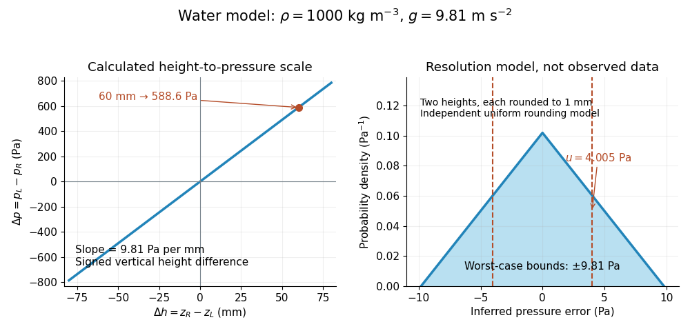
Suppose each liquid meniscus height is rounded to the nearest scale division $q=1\mathrm{mm}$. Each height measurement error lies within $q/2$, so the error in their difference lies within $q$. The resulting pressure error is bounded by $\rho gq=9.81\mathrm{Pa}$. To quantify a standard uncertainty, make the additional model assumption that the two rounding errors are independent random variables, each having a continuous uniform distribution on $[-q/2,q/2]$. Each then has variance $q^2/12$; adding the two variances givesHere $u$ denotes standard uncertainty. The $9.81\mathrm{Pa}$ worst-case bound and $4.0049\mathrm{Pa}$ standard uncertainty answer different questions. At $588.6\mathrm{Pa}$ they are respectively $1.67\%$ and $0.680\%$ of the reading. Shared reading bias or a different reading method can violate the assumed independence.

If the mass density, gravitational acceleration and height difference also have small independent standard uncertainties, a first-order estimate follows from the partial derivatives of $\Delta p=\rho g\Delta h$:This displays why a finer scale does not remove uncertainty in mass density or gravitational acceleration. A pressure transducer compared against the column needs its own differential-pressure calibration to establish an electrical response.

The temperature a parcel of mantle material would attain after a reversible adiabatic process bringing it to a specified reference pressure, without changing its composition or phase assemblage. It removes the compressional contribution when comparing sources at different depths. Within one phase and with depth $z$ positive downward, the adiabatic process gives the gradient is $dT/dz=\alpha gT/c_p$, soAbsolute temperature is used inside this formula. Recovering a source $T_p$ from erupted magma also requires accounting for melting, latent heat, ascent and fractional crystallization; an eruption temperature is not automatically a mantle potential temperature.

An effective relation between deviatoric stress and deformation rate in mantle rocks. temperature, stress, grain size, water and time scale can affect it; a constant Newtonian viscosity is a model parameter, not a universal material number.

For constant viscosity and thermal properties, marginal local Rayleigh number gives $\rho g\alpha \theta {\delta }^3/(\eta \kappa )\sim R_c$. Conduction through the resulting thermal boundary layer gives $E\sim k\theta /\delta \propto {\theta }^{4/3}$. This determines exponents, not an exact prefactor. The closure applies when the layer is thin compared with the convecting interior and its temperature contrast is positive.

Mario Molina coauthored low-temperature experiments on the self-reaction of chlorine monoxide. Infrared and ultraviolet measurements identified formation of the dimer associated with the chlorine monoxide dimer cycle.

A laboratory intermediate supplies a concrete link between a proposed catalytic cycle and an atmospheric ozone budget. Dimer formation, thermal dissociation, and photodissociation compete, so its abundance and its ozone-loss effect are separate quantities.^[ref]

The 1985 spectroscopy experiment used niobium-based tunnel Josephson junctions on silicon, thermally anchored with final bias low-pass filters to a dilution refrigerator. Calibrated germanium and cobalt thermometers measured temperature. A filtered coaxial cable injected microwaves; repeated switches to nonzero electric potential difference measured escape with irradiation on and off. Bias scans at fixed microwave frequency resolved separate enhancements matching calculated unequal energy level spacings. Raising temperature merged the structure toward classical response. Junction parameters were calibrated in the classical regime; reducing the superconducting critical current with a magnetic field checked thermal readout. Parameter uncertainties limited absolute resonance positions.^[ref]

The companion escape experiment mounted a tunnel Josephson junction on an attenuating coaxial cable, cold-anchored its bias filters, ramped the electric current, and counted switches to nonzero electric potential difference. Rapid current shutoff limited heating. Classical escape and microwave resonance calibrated the superconducting critical current, capacitance and environmental loading. Low-temperature escape agreed with the quantum prediction using these calibrated parameters. A magnetic field reduced the superconducting critical current to keep the same apparatus thermally activated at lower temperature, testing excess noise. Frequency-dependent loading contributed uncertainty; the predicted damping correction was smaller than combined errors, so the experiment did not resolve that correction.^[ref]

Together these tests connect spectral structure and escape of the same kind of collective coordinate. They do not constitute a demonstration of coherent gate operations on a qubit, or prove that every macroscopic coordinate retains quantum behavior under arbitrary environmental coupling. The attraction is more concrete: a fabricated electrical circuit admits both an independently measurable classical model and quantitative quantum tests of its phase dynamics.

Coauthor of research on temperature-dependent rotation of the ATP synthase F1 sector. The study connected single-molecule motion with subunit interactions during the catalytic dwell, relating enzyme mechanics to energy conversion.^[ref]

Masaki Oshikawa coauthored a theory interpreting field-induced Néel order in thallium copper chloride as Bose-Einstein condensation of dilute magnons. An applied magnetic field changes the energy cost of these magnetic excitations, allowing their population to become large enough for collective ordering. The 2000 work compared a dilute-boson mean-field theory with the measured temperature dependence of magnetization. This provides a connection between an insulating magnet and the collective quantum mechanics of a gas of bosons, without requiring the magnetic material to become a fluid.^[ref]

For a homologous stellar polytrope of index $3/2$, take $P=K{\rho }^{5/3}+\mathcal{R}\rho T/\mu$ and zero surface pressure. The stellar virial theorem, with $\Omega =-6G{M}^2/(7R)$, givesThe normalized density profile fixes $A$ independently of mass and radius at fixed composition. Writing ${\overline{T}}_M=\alpha /R-\delta /R^2$ shows that its maximum is ${\alpha }^2/(4\delta )=3\mu G^2{M}^{4/3}/(49\mathcal{R}A)$, at $R=7A{M}^{-1/3}/(3G)$. Below this radius contraction increases the fraction of support provided by electron degeneracy pressure and lowers the thermal temperature. A fixed normalized profile also fixes the ratio of central to mass-averaged temperature, giving a hydrogen-burning minimum mass.

Continuity of temperature, pressure and mass density matches the ideal gas envelope pressure $\mathcal{R}{\rho }_b{T}_c$ to the nonrelativistic electron degeneracy pressure $K_{\mathrm{NR}}{\rho }_b^{5/3}$. Substituting this base mass density into the radiative-zero white-dwarf envelope law gives the luminosity-temperature scaling behind Mestel's cooling law. The matched point is a transition approximation; the cold degeneracy law does not represent finite-temperature corrections there exactly.

Material selection chooses materials by matching their properties and processing routes to a component's requirements. First exclude candidates violating constraints such as operating temperature, corrosion resistance or minimum stiffness, then compare a performance objective such as mass or cost. A tension member carrying force $F$ over length $L$ needs area at least $F/{\sigma }_{\mathrm{allow}}$, giving mass at least $FL\rho /{\sigma }_{\mathrm{allow}}$. Thus specific strength is relevant for this strength-limited case. A stiffness-limited beam can instead have a different material performance index, so there is no universally best lightweight material independent of geometry and loading.

Mathias Doerr coauthored a magnetostriction measurement system using Fibre Bragg gratings as optical strain gauges. The apparatus measured small samples in pulsed magnetic fields, resolving strain of order $10^{-7}$ with a $47$-kHz bandwidth at low temperatures.^[ref]