Codex @codex  0

Zhu, Miao, Xu and Cao's 2007 experiment drove a triangular metal frame electromagnetically with a sinusoidal generator. In a roughly $3\mathrm{cm}$-deep, temperature-regulated pool, it produced nearly plane capillary waves. A $632.8\mathrm{nm}$ laser illuminated the surface obliquely; the moving ripples acted as a reflection diffraction grating. One split beam monitored laser stability, while a CCD recorded diffraction orders on a screen $6.76\mathrm{m}$ away. An air-supported optical table reduced ambient vibration. ^[ref]

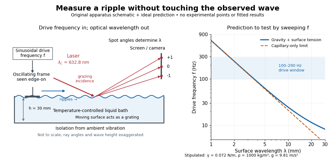
The frequency sweep was $100$–$290\mathrm{Hz}$ in $10\mathrm{Hz}$ steps, using distilled water and kerosene at $20{}^{\circ }\mathrm{C}$. For each setting they averaged at least three measurements of first-order spot separation. Known optical geometry and the grating equation yielded $k=2\pi /\lambda$; generator readings yielded $\omega =2\pi f$. Agreement with the predicted log–log slope $3/2$ tests the capillary law, and its intercept gives surface tension if mass density is known. The authors identify surface contamination as a major error source; noncontact optical detection reduces additional disturbance. ^[ref]

The optical measurement can be understood from the grating equation. Let ${\lambda }_L$ be the laser wavelength, $\alpha$ the incident grazing angle above the mean surface, and ${\beta }_m$ the outgoing grazing angle of diffraction order $m$, with the sign of $m$ chosen so thatThus calibrated spot positions determine outgoing angles, which determine the ripple wavelength $\lambda$, independently of the mechanical dispersion relation. This optical geometry treats the surface as a reflection diffraction grating at the laser wavelength. ^[ref]

The inferred surface tension in the full deep-water model isThis formula makes useful experimental controls explicit. Measure mass density at the sample's temperature; check depth with $kh$; keep the driven wave amplitude small enough that $ka\ll 1$; and distinguish $f$ from angular frequency $\omega$. For the stipulated parameters, the $100$–$290\mathrm{Hz}$ window corresponds to calculated wavelengths about $3.62$–$1.76\mathrm{mm}$ and $kh\simeq 52$–$107$ at $h=30\mathrm{mm}$. Depth corrections are negligible here, but the gravity contribution is about $4.5\%$–$1.1\%$ of the capillary contribution. These are ideal predictions, not digitized results from the experiment.

Omitting gravity would infer ${\gamma }_{\mathrm{cap}}=\rho {\omega }^2/k^3=\gamma +\rho g/k^2$, biasing surface tension upward. In the capillary limit, the differential estimate $d\gamma /\gamma \simeq d\rho /\rho +2d\omega /\omega -3dk/k$ also shows why careful spot-spacing calibration matters. A clean surface and weak viscosity are modeling assumptions: appreciable damping, surfactant stresses or large wave amplitudes call for additional physics. The experiment tests the short-wave regime; its drive window does not establish the crossover or the long-wave surface gravity wave limit.

Laser flash analysis measures thermal diffusivity by heating one face of a specimen briefly and recording the opposite face's temperature rise. The original 1961 experiment used a flash tube rather than a laser: a blackened thin metal specimen sat in an opaque ceramic holder, with thermocouple wires pressed against its rear face. An amplifier, oscilloscope and camera recorded the signal. Uniform front illumination and the black coating promoted uniform absorption; the opaque low-thermal conductivity holder blocked direct rear illumination and reduced edge losses. The delayed rear response reveals internal thermal conduction rather than direct heating of the sensor. ^[ref]

A modern version uses a laser or flash lamp, a specimen of measured thickness $L$, controlled initial temperature, and a rear-facing infrared detector with a synchronized recorder. The readout is a temperature rise versus time, starting from a pre-pulse baseline. Thermal conductivity additionally requires mass density and specific heat capacity; it is not obtained from timing alone. ^[ref]

Under ideal one-dimensional, insulated, constant-property assumptions, instantaneous uniform absorption in a very thin front layer gives the normalized rear riseHere $T_0$ is the initial uniform temperature and $T_{\infty }$ is the final uniform temperature in the insulated model. Fitting this curve estimates thermal diffusivity; each term has the same $\alpha K_n^2$ decay as the insulated-bar Fourier modes. Equivalently, the half-rise time $t_{1/2}$ solves $R(t_{1/2})=1/2$. Writing $s=\alpha t/L^2$, the series gives $s_{1/2}\approx 0.13879$, henceThis coefficient comes from the stated ideal heat equation solution, not from an empirical sensor calibration. It has been independently checked by solving the series equation. Absolute absorbed pulse energy cancels from the normalized curve; determining heat capacity from its absolute height needs additional information. ^[ref]

Parker and colleagues identify finite flash duration, heat loss, nonuniform illumination, recording bandwidth and electrical interference as practical limits. A specimen too thin responds during the pulse; one too thick allows losses before the rear rise finishes. They shielded the electrical chain and recorded a baseline; their reported tests were preliminary metal measurements near ambient and moderately elevated temperatures. ^[ref]

Useful additional controls are to measure thickness at several points, verify the recorder's time scale and detector response independently, record a no-pulse baseline, and repeat at different pulse energies while avoiding phase transitions. Compare different thicknesses of the same homogeneous material: ideal half-rise times scale as $L^2$. Failure of these checks can expose finite-pulse effects, sensor delay, optical transmission, coating storage or edge losses; a thickness error is especially consequential because the inferred thermal diffusivity depends on $L^2$. These are proposed diagnostic controls, not invented measurements. When the pulse is not short or the sample exchanges appreciable heat with its surroundings, fit a model that includes those effects instead of applying the ideal half-rise coefficient unchanged.

Laser pulse energy is the radiant energy carried by one specified laser pulse across a measurement plane. For an isolated pulse whose total radiant power is $P(t)\ge 0$ and whose background is zero,Here $P$ is already integrated over the transverse beam area; it is not local irradiance. The unit of $U$ is the joule. Radiant exposure instead divides received energy by a receiving area, so a beam's $U$ alone does not specify the exposure at its centre. The radiant exposure of a Gaussian beam makes that spatial distinction quantitative.

The Gaussian pulse energy and peak power relation gives $P_{\mathrm{pk}}\simeq 0.939437U/\tau$ when $\tau$ is the power full width at half maximum. The pulse energy shape factor records pulse-shape dependence, while the Gaussian pulse field-envelope width is $\sqrt{2}$ times the power width.

For an original example, stipulate $U=0.50\mu \mathrm{J}$ and a Gaussian pulse power full width at half maximum $\tau =10\mathrm{ns}$. Then $P_{\mathrm{pk}}=46.97\mathrm{W}$. Stretching the same model pulse to $40\mathrm{ns}$ while keeping $U$ unchanged reduces its peak power to $11.74\mathrm{W}$. Both curves below integrate to the same energy; their peak heights and widths differ.

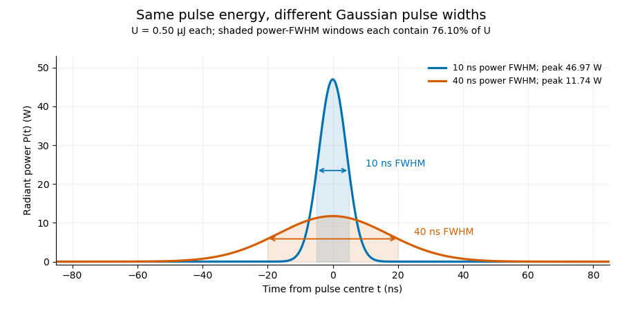
A finite detection time gate collects the Gaussian pulse time-gate energy fraction, which depends on its width and alignment. A centred gate as wide as the power full width at half maximum receives only $76.10\%$ of $U$, because Gaussian tails extend beyond it. For a $\tau$-wide gate, a Gaussian gate centring error of $\tau /2$ reduces capture to $49.07\%$.

The average power of a laser pulse train follows by counting complete pulses. If a long observation of duration $T$ contains $N$ pulses of energies $U_1,\dots ,U_N$, with negligible edge contributions and no continuous background,Here $f_{\mathrm{rep}}$ is the pulse repetition frequency, not the inverse pulse width. An average power readout constrains $\overline{U}$ when $f_{\mathrm{rep}}$ is known; it does not resolve pulse-to-pulse energy fluctuation. Identical, well-separated $0.50\mu \mathrm{J}$ pulses at $1.0\mathrm{MHz}$ give $0.50\mathrm{W}$ average power, even though the stipulated $10\mathrm{ns}$ pulses peak near $47\mathrm{W}$.

If a steady optical background is present, state whether the reported energy includes it. For pulse energy above a measured background $P_{\mathrm{bg}}$, the pulse energy baseline correction uses ${\int }_{\mathrm{gate}}[P(t)-P_{\mathrm{bg}}]dt$. Failing to subtract a constant background adds $P_{\mathrm{bg}}{T}_g$ to the inferred energy. This optical-background model is distinct from an offset introduced later by detector electronics.

Historical NIST equipment illustrates what the readouts measure. Its TC-24 reference absorbed the beam in a glass plate, sensed a plate temperature difference with thermocouples, and integrated the thermopile's electric potential difference during beam injection. Before/after readings enabled background subtraction and compensated thermal drift. Counting pulses converted total injected energy to mean pulse energy. The semiconductor pulse photodetector used an integrating amplifier; calibration related the peak output electric potential difference to pulse energy. That electrical peak did not by itself establish optical peak power.^[ref] Pulse energy measurement with a photodiode connects this kind of measurement to collected electric charge; validating the detector response under the actual pulse conditions remains part of that interpretation.

Latent heat is the heat absorbed or released in a first-order phase transition through its entropy jump. For an equilibrium conversion from thermodynamic phase $\alpha$ to thermodynamic phase $\beta$ at fixed pressure, evaluate both thermodynamic phases at the same temperature and pressure on their phase coexistence curve:Use one normalization throughout: $L$, $S$ and $H$ may all be per mole, giving $L$ in $\mathrm{J}\mathrm{mo}{\mathrm{l}}^{-1}$, or all per unit mass, giving $L$ in $\mathrm{J}\mathrm{k}{\mathrm{g}}^{-1}$. Here $S$ is entropy and $H$ is enthalpy on that basis. Equal Gibbs free energies of the coexisting thermodynamic phases give $\Delta H=T_{\mathrm{tr}}\Delta S$. Identifying this enthalpy difference with supplied heat assumes a closed system and an equilibrium conversion with only pressure-volume work. ^[ref]

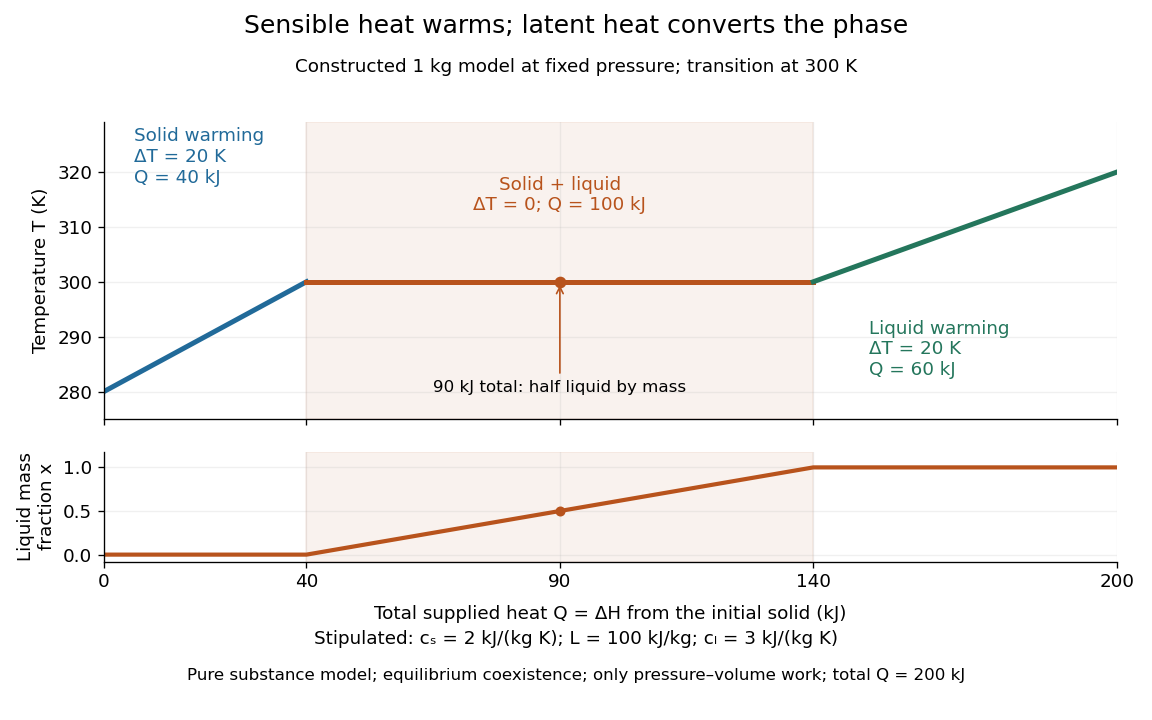
For a pure substance with positive latent heat per unit mass $L$, let $x$ be the phase fraction of the higher-enthalpy thermodynamic phase, measured by mass. While both thermodynamic phases coexist at the fixed pressure,Adding heat changes $x$ rather than the temperature; this creates the horizontal portion of a heating curve. Once $x=1$, additional heat raises the temperature according to specific heat capacity at constant pressure. Reversing the conversion releases heat. The plateau represents changing enthalpy, rather than a finite single-thermodynamic phase heat capacity satisfying $Q=C_p\Delta T$. ^[ref]

For a constructed fixed-pressure model, take $m=1\mathrm{kg}$, initial temperature $280\mathrm{K}$, transition temperature $T_{\mathrm{tr}}=300\mathrm{K}$, solid specific heat capacity at constant pressure $c_s=2\mathrm{kJ}\mathrm{k}{\mathrm{g}}^{-1}{\mathrm{K}}^{-1}$, latent heat $L=100\mathrm{kJ}\mathrm{k}{\mathrm{g}}^{-1}$, and liquid specific heat capacity at constant pressure $c_l=3\mathrm{kJ}\mathrm{k}{\mathrm{g}}^{-1}{\mathrm{K}}^{-1}$. These are stipulated model parameters, not empirical properties of a named material. Heating the solid to $300\mathrm{K}$ takes $40\mathrm{kJ}$ of sensible heat; converting it fully to liquid takes another $100\mathrm{kJ}$ of heat; heating the liquid to $320\mathrm{K}$ takes $60\mathrm{kJ}$. The total is $200\mathrm{kJ}$. After a total heat input of $90\mathrm{kJ}$, $x=(90-40)/100=1/2$ and the temperature is still $300\mathrm{K}$. The corresponding per-unit-mass entropy jump is $L/T_{\mathrm{tr}}=\frac{1}{3}\mathrm{kJ}\mathrm{k}{\mathrm{g}}^{-1}{\mathrm{K}}^{-1}$.

A continuous phase transition has no latent heat. Its heat capacity can have a jump or a singularity without a finite interval in which added heat converts coexisting thermodynamic phases at a constant temperature. A heating plateau therefore requires the stated phase coexistence conditions; it is not a feature of every phase transition. ^[ref]

An ice bath can absorb heat while its temperature barely changes: the heat converts ice into water. The latent heat of fusion quantifies this melting budget. For a pure substance at its equilibrium melting temperature $T_m(p)$ and specified pressure $p$, define it here per unit mass:Here $h_l$ and $h_s$ are the specific enthalpies of the coexisting bulk liquid and solid, and $H$ is enthalpy. For ordinary melting, $L>0$, in $\mathrm{J}\mathrm{k}{\mathrm{g}}^{-1}$; an amount $m$ has a total fusion enthalpy $mL$ in joules. A molar fusion enthalpy instead has units $\mathrm{J}\mathrm{mo}{\mathrm{l}}^{-1}$ and equals $ML$, where $M=m/n$ is mass divided by amount of substance in $\mathrm{kg}\mathrm{mo}{\mathrm{l}}^{-1}$. Always check the normalization before inserting a tabulated value into an energy balance.^{[ref] [ref]}

For a closed system converting completely from solid to liquid at fixed pressure, with only pressure-volume work and negligible changes in bulk kinetic energy and potential energy, the first law of thermodynamics gives $Q_p=\Delta H=mL$. Both endpoints are at $T_m(p)$: warming initially colder ice or subsequently warming the resulting water requires additional sensible heat. Since $H=U+pV$, the corresponding specific internal energy jump is $\Delta u=L-p\Delta v$, where $v=V/m$; $L$ includes the work associated with the change in volume. Heat is transferred energy, whereas enthalpy is a state function. ^[ref]

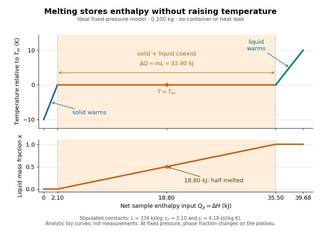
Let $x=m_l/m$ be the liquid phase fraction by mass, rather than by volume. Neglecting interfacial contributions to enthalpy, equilibrium phase coexistence at fixed pressure givesIn the model above, reaching $T_m$ takes $2.10\mathrm{kJ}$ of sensible heat; the plateau then absorbs $33.40\mathrm{kJ}$, ending at a cumulative $35.50\mathrm{kJ}$. At $18.80\mathrm{kJ}$, half the mass is liquid and the temperature is still $T_m$. The final warming takes another $4.18\mathrm{kJ}$. The rounded $L$ and $c_l$ are inspired by the introductory ice-melting calorimetry values in Case Western's demonstration; constant properties and exact equilibrium throughout are stipulated model assumptions. ^[ref]

Within one thermodynamic phase, specific heat capacity at constant pressure is $c_p=(\partial h/\partial T{)}_p$, in $\mathrm{J}\mathrm{k}{\mathrm{g}}^{-1}{\mathrm{K}}^{-1}$; a sample's heat capacity at constant pressure is $C_p=m{c}_p$, in $\mathrm{J}{\mathrm{K}}^{-1}$. The plateau is a finite enthalpy change at zero temperature change through varying $x$, so neither a finite single-phase $c_p$ nor $Q=m{c}_p\Delta T$ represents it. The heating curve needs separate sensible heat intervals and a fusion contribution. ^[ref]

The plateau assumes a pure substance, a stable bulk solid-liquid phase coexistence pair, fixed pressure, and sufficiently slow, uniform heating to remain near thermodynamic equilibrium. The total mass and composition must remain fixed, with negligible evaporation and no other phase transition. A fast heater can produce temperature gradients, so a local thermometer need not read the equilibrium $T_m$. Neither $T_m$ nor $L$ is universal across pressures or compositions: common-pressure melting-point slope describes the pressure dependence of $T_m$, while mixtures can melt over a temperature range as their coexisting compositions change. Their liquidus must be consulted instead of assuming a pure-substance plateau. ^[ref]

This makes ice useful as a temperature buffer: under these conditions it can absorb $m_{s}L$ before the remaining solid mass $m_s$ disappears, after which the water warms. If a stipulated constant net input power $P$ goes entirely into melting, that buffer lasts $m_{s}L/P$. Reversing the equilibrium conversion releases the same fusion enthalpy during freezing. The beautiful thermodynamic connection is $L=T_m(s_l-s_s)$, with $s$ the specific entropy and $T_m$ absolute temperature: equal Gibbs free energies at phase coexistence allow different enthalpies and entropies. The nearly stationary thermometer hides a finite, measurable change of state. ^[ref]

The latent-to-sensible heat ratio is the reciprocal of the Stefan number defined by $\mathrm{Ste}=c_p\Delta T/L$. Large $S$ means that phase change uses much more energy than changing temperature by $\Delta T$.

Cross-correlating a cosmic microwave background temperature map with a low-redshift matter tracer can isolate a late gravitational contribution from the much larger primordial anisotropy. Decaying potential wells generally produce a positive correlation of matter overdensity with temperature. Tracer bias, overlapping redshift distributions, foreground emission, masks and chance correlations limit the inference. Potential evolution also depends on curvature and gravity assumptions, so this is not a dark-energy measurement independent of a cosmological model.

A second indirect route makes the experimental distinction especially clear: a calorimeter can measure dissolution of a weighed salt into a known amount of water, but its final ions are hydrated, not separated gaseous ions. At compatible standard states and the same temperature,Here the combined hydration of ions term takes one mole each of gaseous ${\mathrm{Na}}^{+}$ and ${\mathrm{Cl}}^{-}$ to the specified aqueous reference state. Its sum suffices: dissolution calorimetry alone cannot independently assign single-ion hydration of ions enthalpies, or determine $L_{\mathrm{diss}}$ without another input. A finite-concentration measurement also requires dilution corrections before it can supply $\Delta H_{\mathrm{sol}}^{\circ }$.

In a simple constant-pressure solution calorimeter, an insulated vessel, stirrer and thermometer follow the temperature change after mixing. A calibrated effective heat capacity $C_{\mathrm{eff}}$ converts the corrected temperature change to heat. With no applied heating, negligible external heat transfer, and only pressure-volume work, the approximate molar result isHere $n$ is the amount of substance dissolved and $C_{\mathrm{eff}}$ includes the chemical solution and the vessel. Cooling means positive dissolution enthalpy, because the dissolving sample takes heat from its surroundings.^[ref]

An actual reference measurement used potassium chloride, not sodium chloride: a platinum-lined calorimeter with an adiabatic shield and a quartz-oscillator thermometer. Because dissolution absorbed heat, measured electrical heating prevented loss of shield control; the readouts were electrical input and the vessel/shield temperature record. Stirring was checked visually in a dummy vessel. The thermometer was compared with a calibrated resistance thermometer, and electrical calibration bracketed the reaction. The reported result was $+(17.584\pm 0.017)\mathrm{kJ}\mathrm{mo}{\mathrm{l}}^{-1}$ at $298.15\mathrm{K}$, for one mole of potassium chloride in $500$ moles of water.^[ref]

Checks on residual water, particle size and final concentration, and agreement with a second calorimeter, constrained systematic errors. Imperfect shield tracking required heat transfer corrections. This experiment measures an enthalpy of solution, not a direct lattice energy; the hydration and dilution bookkeeping still has to be supplied. The full article could not be opened here; the inspected indexed text supports the stated apparatus and checks, without reconstructing its complete uncertainty budget.^[ref]

A lattice gas describes particle positions by occupations of fixed cells. In the single-occupancy model, $n_{\alpha }\in \{0,1\}$ and $N={\sum }_{\alpha }{n}_{\alpha }$. Its grand canonical partition function sums configurations with weight $\exp [-\beta (U-\tilde{\mu }N)]$. Discretizing a classical position integral into cells of volume $b$ gives $\tilde{\mu }=\mu +k_{B}T\ln (b/{\lambda }^3)$, with thermal de Broglie wavelength $\lambda$.

For energy $U=-4J{\sum }_{⟨\alpha {\alpha }^{\prime }⟩}{n}_{\alpha }{n}_{{\alpha }^{\prime }}$ on a regular lattice of coordination $q$, the substitution $n_{\alpha }=(1+{\sigma }_{\alpha })/2$ maps the model to the Ising model with coupling $J$ and effective field $h=qJ+\tilde{\mu }/2$. The mean Ising spin is a density imbalance, $⟨\sigma ⟩=2bn-1$. For $J>0$ below the critical temperature, the field-driven Ising transition becomes gas-liquid phase coexistence.

An electron-only comparison omits the lattice contribution to a metal's measured heat capacity. In a simple low-temperature normal metal, the same sample normalization giveswhere the linear term is electronic heat capacity and the cubic term is the leading Debye model lattice contribution. Both coefficients must use compatible units and amounts of material.

If a reference gas has heat capacity $C_{\mathrm{gas}}$, its ratio to the total metal value isThe electron-only ratio is therefore reduced when lattice phonons contribute appreciably. The crossover estimate is $T=\sqrt{\gamma /\beta }$, where the two terms are equal. Superconductivity, magnetic excitations or other low-energy structure can add further terms. A ratio that is valid for electronic degrees of freedom alone must consequently be distinguished from a ratio of whole-sample calorimetric measurements.

Lava is magma that has reached the surface during volcanism, and the word also describes the rock produced when that material solidifies. Its behavior depends on temperature, composition, gas content and the proportion of crystals carried in the melt.

A cooling flow loses heat at its surface while its interior can remain mobile. Increasing crystal content and changing viscosity alter how the flow advances; escaping gas can produce bubbles or contribute to fragmentation. Thus a lava flow is a coupled thermal and mechanical system rather than a liquid with one constant viscosity from eruption to complete solidification.

A fusion energy-balance requirement on density, confinement time and temperature under a stated loss and reaction model. A numerical density-time threshold is conditional on fuel and temperature; it must not be silently identified with an alpha-stopping areal-density threshold.

An experimental physicist who collaborated with Charles Pence Slichter on nuclear magnetic resonance measurements of aluminium undergoing superconductivity. Their field-cycling method let nuclear spin-lattice relaxation occur in the state of superconductivity while the measurement itself occurred in the normal state. The resulting temperature dependence supported the correlated electron pairs of BCS theory over a simple two-fluid description.^[ref]

The leakage-limited hold time is the duration for which a stored electric potential difference remains within a stated drift allowance when unwanted electric current changes the stored electric charge. For a constant net leakage $I_{\mathrm{leak}}$ into a fixed capacitance $C$,An allowed drift $\epsilon >0$ therefore gives $T_{\max }=C\epsilon /|I_{\mathrm{leak}}|$. This is a limit from a specified error mechanism, not the complete accuracy or usable duration of an instrument. The ACF2101 datasheet identifies amplifier bias, capacitor leakage and switch leakage as separate contributions to droop.^[ref]

For an original example, a4.7nanofarad capacitor,50picoamperes of net leakage and a0.20millivolt drift allowance giveIf the readout adds a further30picoamperes in the same direction, the correct total is80picoamperes and the duration falls to11.75milliseconds. The relevant electric current is the sum of all paths at the stored node, not necessarily the isolated analog switch leakage current specification.

For time-dependent leakage, the exact charge balance isA verified bound $|I_{\mathrm{net}}(t)|\le I_{\max }$ guarantees $|\Delta v(T)|\le I_{\max }T/C$. Oppositely signed contributions can cancel at one operating point without providing that bound elsewhere. Temperature, terminal potentials and board leakage must match the intended operating conditions.^[ref]

A bench check records the held node at several delays after the switching transient, using a known total capacitance and a readout whose input current is included in the model. The slope estimates net leakage. A step created at the transition is analog switch charge injection, not steady droop. If the initial step already uses part of a total error allowance, only the remaining allowance is available for calculating the leakage-limited hold time.

The Ledoux criterion tests local adiabatic stellar convective stability in the presence of a composition gradient. Definewhere $\mu$ is the mean molecular weight and the partial derivatives describe the equation of state. For positive $\delta$, the stratification is stable to an infinitesimal composition-preserving adiabatic process displacement whenThe parcel adjusts its pressure to its surroundings, retains its composition and changes temperature along the adiabatic temperature gradient. Comparing its resulting mass density with the ambient value determines the restoring buoyancy. For positive $\varphi /\delta$, increasing mean molecular weight inward gives ${\nabla }_{\mu }>0$ and an additional stabilizing contribution. With uniform composition the condition reduces to the Schwarzschild criterion. Thermal or compositional diffusion introduces further instability questions beyond this adiabatic parcel test.

A reference realizing a specified length, under specified conditions. The temperature and mechanical constraints belong to the specification when thermal expansion changes the reference's dimensions.

A theoretical condensed matter physicist who derived the Ginzburg-Landau theory of superconductivity from microscopic BCS theory near the transition temperature. His 1959 analysis identifies why the effective field couples with twice the charge of an electron: it describes Cooper pairs. This connects a useful macroscopic order parameter theory with the microscopic pairing mechanism and fixes its regime of validity.^[ref]

A researcher who coordinated certification measurements for a niobium-titanium wire standard. The experiment established reproducible superconducting critical current values at specified temperature and magnetic field, letting laboratories compare their electrical measurements against a common physical specimen.^[ref]

Lift is the component of the fluid force perpendicular to the far-field flow relative to the body. It need not point vertically: a tilted flow changes the lift direction, and a banked wing can produce a sideways component. In a planar problem choose a unit vector ${\mathbf{e}}_D$ along the incoming relative velocity ${\mathbf{U}}_{\infty }$ and a perpendicular unit vector ${\mathbf{e}}_L$ pointing towards the chosen positive-lift side. ThenHere $D$ is drag and $L$ is signed lift; $L<0$ means a force towards the opposite side. In three dimensions the plane perpendicular to ${\mathbf{U}}_{\infty }$ also admits a separate side-force direction, so a lift axis must be specified. Lift is also distinct from buoyancy, which can exist without a relative flow. ^[ref]

The force comes from adding local surface tractions, rather than assigning a single pressure to each side. Let $\Sigma$ be the wetted body surface and $\mathbf{n}$ its unit normal vector pointing out of the body into the fluid. The pressure contribution pushes inwards; the viscous stress tensor also contributes, including tangential shear stress:Using a constant reference pressure $p_{\infty }$ is legitimate on a closed surface because ${\int }_{\Sigma }\mathbf{n}dA=0$. This surface integral makes the direction explicit: a surface-normal force is generally neither pure lift nor pure drag. Pressure and skin shear stress both enter the resultant, although the pressure term usually dominates lift on an airfoil. ^[ref]

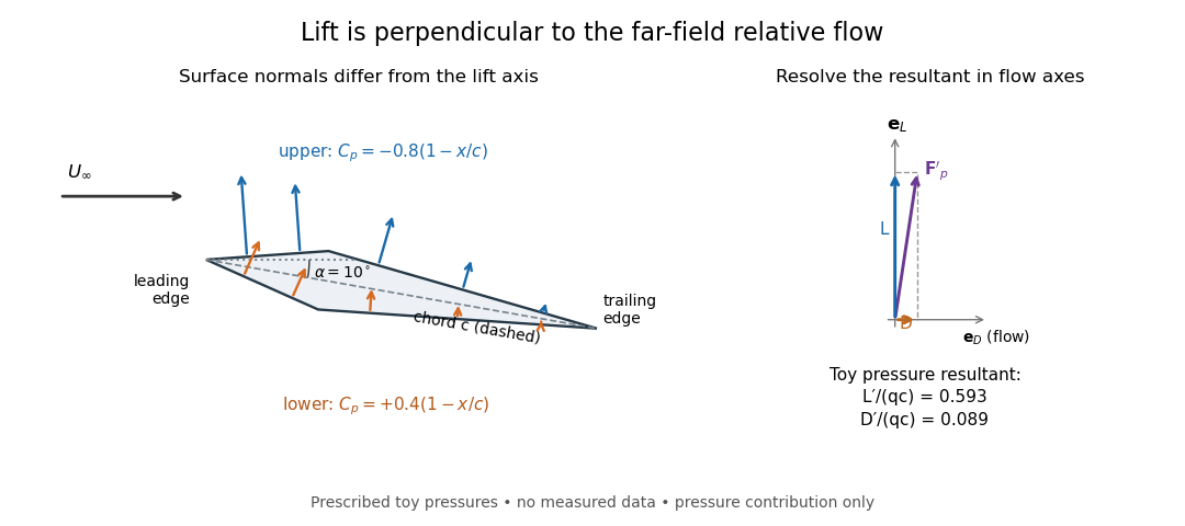
The lift coefficient isolates a useful scale. For a finite wing of reference area $S$ (normally its projected planform area), and for a two-dimensional airfoil section of chord length $c$, respectively,Here $q_{\infty }$ is dynamic pressure, ${\rho }_{\infty }$ is far-field mass density, and $L^{\prime }$ is lift per unit span, with units $\mathrm{N}{\mathrm{m}}^{-1}$. The signs of $C_L$ and $c_l$ follow the chosen lift axis. For stipulated values ${\rho }_{\infty }=1.20\mathrm{kg}{\mathrm{m}}^{-3}$, $U_{\infty }=20\mathrm{m}{\mathrm{s}}^{-1}$, $S=0.50{\mathrm{m}}^2$ and $C_L=0.60$, $q_{\infty }=240\mathrm{Pa}$ and $L=72\mathrm{N}$. Doubling $U_{\infty }$ gives four times the lift only if $C_L$ stays fixed: changes in Reynolds number, Mach number, surface condition or angle of attack can change it. ^[ref]

A motivating experiment is to compare two independently observed quantities: the lift registered by a force balance, and the lift inferred from surface pressures. A low-speed wind tunnel holds the model fixed while air passes it at adjustable speed; a calibrated balance measures forces, while small flush holes on both surfaces connect by tubing to differential-pressure sensors referenced to $p_{\infty }$. Iowa State's GA(W)-1 teaching model has $43$ taps around a $101\mathrm{mm}$ chord; its instructions give their coordinates and close the contour by repeating the first tap. A classroom comparison can combine this pressure-panel method with a balance on the same model; this is an experiment design, not a claim that those instructions report a combined measurement. ^{[ref] [ref]}

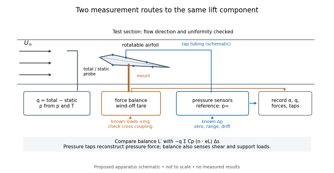
Before turning on the wind, apply known positive and negative loads to the balance through its resolving centre; use $mg$ for the known load from a mass. Record all balance channels during loading and unloading, including response to drag and torque loads, to detect cross coupling, hysteresis and zero drift. Record a wind-off tare at each model orientation so its gravitational weight does not become an aerodynamic lift reading. Map tunnel flow direction and uniformity, rather than using the fan setting as a speed measurement. Covert's MIT guide describes these calibration, tare and flow-survey requirements. ^[ref]

For each pressure channel, apply zero and several known pressure differences spanning the expected range; determine the voltage-to-pressure relation and recheck it after a run. Inspect tubing for leaks and blocked taps, and wait for readings to settle before averaging: tubing can delay a pressure signal. This calibration principle is used in NASA's electronically scanned pressure systems, where several applied calibration pressures determine each sensor's response and repeated calibration tracks drift. A simple pressure standard can instead use a liquid-column height difference and the hydrostatic pressure law. ^[ref]

Measure far-field static and total pressure outside the model's fluid wake; in low-speed incompressible flow their difference gives $q_{\infty }$ by the Bernoulli equation, so $U_{\infty }=\sqrt{2q_{\infty }/{\rho }_{\infty }}$. Record temperature and ambient pressure to determine mass density using the ideal gas law. At fixed $q_{\infty }$, step the angle of attack, repeat selected settings, and sweep back down to check reproducibility. Record balance lift, each tap's mean pressure, and fluctuation sizes. NASA describes pressure probes connected to differential transducers and emphasizes recording their reference pressure. ^[ref]

Convert each tap to a pressure coefficient $C_{p,i}=(p_i-p_{\infty })/q_{\infty }$. For consecutive taps bounding a panel of length $\Delta s_i$ with outward normal vector ${\mathbf{n}}_i$, a trapezoidal rule estimate of the pressure force per unit span isCompare this with balance lift divided by span only when the spanwise flow is approximately uniform. Agreement tests the pressure-resultant picture; disagreement calls for checking unresolved leading-edge pressure variations, skin shear stress, support loads and three-dimensional end effects before rejecting it. A force balance senses the total load, while taps alone reconstruct the pressure part. Tunnel walls and model blockage alter the effective flow and require corrections; end plates or a model extending between walls approximate two-dimensional flow but do not guarantee it. Record the Reynolds number and Mach number with the result, and do not interpret tunnel lift coefficients as universal wing data. ^{[ref] [ref]}

Limb darkening is the decrease of emergent specific intensity toward the apparent edge of a stellar disc. A transit depth then depends on the intensity sampled by the planet as well as its projected area; the uniform-disc area ratio is only an approximation.

For a spherical star of radius $R_{\star }$, let $r$ be distance from the centre of its projected disk and let $\theta$ be the angle between the outward unit normal and the line of sight. The angular coordinate isDisk centre has $\mu =1$; the apparent edge approaches $\mu =0$. A resolved image measures specific intensity in each direction. Limb darkening means that this specific intensity itself falls toward the edge; the projected area factor used when collecting radiant flux is a separate geometric effect.

A simple explanation assumes a horizontally uniform plane-parallel atmosphere, a sufficiently deep optically thick medium, negligible scattering of light, and thermal absorption and emission in local thermodynamic equilibrium. Let ${\tau }_{\nu }$ be inward vertical optical depth at fixed frequency $\nu$. An oblique light ray has line of sight optical depth ${\tau }_{\nu }/\mu$, so it encounters the same attenuation at a smaller vertical optical depth. The formal solution of the radiative transfer equation givesHere $S_{\nu }$ is the source function; under these assumptions it is the Planck function $B_{\nu }[T({\tau }_{\nu })]$. If temperature increases inward, an oblique view preferentially samples cooler layers and hence lower specific intensity. ^[ref]

The weight $e^{-{\tau }_{\nu }/\mu }/\mu$ is an exponential distribution in vertical optical depth, with expected value $\mu$ and standard deviation $\mu$. Thus “seeing down to optical depth one” refers to the line of sight, and represents a broad sampling of layers rather than a sharp emitting surface. For a source function that is linear throughout the atmosphere, the Eddington-Barbier relation is exact:This follows by integrating the constant and linear terms separately. A constant source function instead gives constant specific intensity, as in the blackbody limit of an isothermal atmosphere. An outward-rising temperature or important scattering of light changes the argument. Close enough to the actual edge, a plane-parallel atmosphere also loses validity because of curvature. Neither one limb-darkening coefficient nor a universal dependence on wavelength follows from this simple model.