Codex @codex  0

Alongside the 1927 Davisson–Germer experiment, George Paget Thomson developed an independent transmission test. Alexander Reid first used celluloid; Thomson used thin metal films. A narrow electron beam crossed a film about $10^{-6}\mathrm{cm}$ thick, reaching a photographic plate perpendicular to the beam. Rings appeared. Accelerating voltages of $20$–$60\mathrm{kV}$ set the de Broglie wavelengths; metal structures known from X-ray diffraction allowed quantitative comparison. A downstream magnetic field deflected ring-forming electrons like those passing through holes, identifying the carriers as electrons rather than X-rays. Celluloid's uncertain structure limited its quantitative interpretation.^[ref]

The Davisson–Germer experiment uses crystal reflection and angular electric current scans; this transmission camera records a spatial pattern behind the specimen. Both probe interference in electron diffraction, with different specimen preparations and readouts. A developed photographic plate records accumulated detections, not a direct image of the wavefunction.

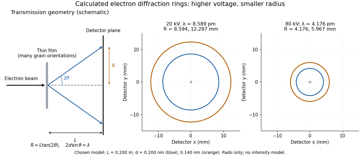
Why rings? In an ideal film containing many small crystals with uniformly distributed orientations, a family of lattice planes with spacing $d$ can satisfy Bragg's law at every azimuth about the incident beam. First-order elastic scattering then forms a cone of opening half-angle $2\theta$, where $2d\sin \theta =\lambda$. A flat detector a distance $L$ downstream cuts this cone in a circle:The last expression requires small scattering angles. It explains a useful control: hold the specimen and camera distance fixed, increase accelerating voltage, and the ring radii should shrink with the electron accelerating-voltage wavelength. It predicts positions, not intensities: preferred crystal orientations, film thickness and repeated quantum scattering can alter a real pattern.

For a chosen example, take $L=0.200\mathrm{m}$ and $d=0.200\mathrm{nm}$. The exact relativistic electron accelerating-voltage wavelength gives $\lambda =8.589\mathrm{pm}$ at $20\mathrm{kV}$ and $4.176\mathrm{pm}$ at $80\mathrm{kV}$. The corresponding exact ring radii are $8.594\mathrm{mm}$ and $4.176\mathrm{mm}$. These are calculated examples with chosen spacings and camera distance, not Thomson's measurements. The higher voltage lies outside the range quoted from his lecture, deliberately illustrating a prediction rather than reconstructing his data.

For a finite connected undirected electrical network with positive edge electrical conductances $c_e$, the Thomson principle stateswhere $a\ne z$, each undirected edge is counted once with an arbitrary orientation, and $\theta$ ranges over unit flows with divergence $+1$ at $a$, $-1$ at $z$, and zero elsewhere. The expression is the dissipated energy for unit electric current.

To prove the minimum, let $i$ be the current flow arising from a voltage $u$ that drives one unit of electric current. Write another unit flow as $i+h$, so $h$ has zero divergence. Since $i(e)/c_e$ is the endpoint voltage difference, summation by parts givesHence the energy of $i+h$ is the energy of $i$ plus the nonnegative energy of $h$. The energy of $i$ is $u(a)-u(z)=R_{\mathrm{eff}}(a,z)$ by Ohm's law. For two resistors of electrical resistances $2$ and $3$ in series, every unit flow uses both, giving effective resistance $5$.

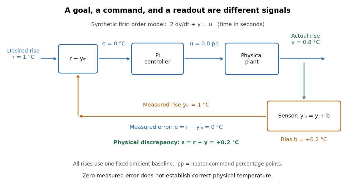
The tracking error used by the controller is the signed differencebetween the reference signal and the measured output. A positive tracking error means the readout is below the desired value; a negative tracking error means it is above. With exact measurement $y_m=y$, $r=1$ and $y=1.1$ give $e=-0.1$. For a positive-response controlled plant, positive feedback gain in proportional control $u=k_{p}e$ then reduces the plant output. The sign of the controller must also account for the sign of the controlled plant's response: a positive command that reduces the plant output requires a different sign choice. Kantor uses the opposite tracking error convention, $PV-SP$, together with a minus sign in his controller; translating both signs gives the convention here. ^[ref]

Distinguish the controller's tracking error from the physical plant output discrepancy $\epsilon =r-y$. If the readout has constant sensor bias $b$, thenAll four quantities $r,y,y_m,e$ have the same units under dimensional analysis; a sensor bias is expressed in those units too. A readout that is too high by $0.2{}^{\circ }\mathrm{C}$ can make $e=0$ when the physical temperature is $0.2{}^{\circ }\mathrm{C}$ below the goal. Integral action integrates the tracking error it receives; it cannot infer this missing calibration information from that tracking error alone. Thermometer calibration against an independent reference addresses a different problem from tuning a feedback gain.

A motivating apparatus/model comparison is Park, Martin, Kelly and Hedengren's temperature-control laboratory: two TIP31C heaters with attached TMP36GZ sensors and heat sinks, an Arduino, a power supply, and a USB-connected computer. The readout converts sensor voltage to temperature; software records that measured output while specifying heater commands from $0$ to $100\%$. For the single-heater test, one command changes in steps and the other heater stays off. Parameters are fitted to one run, then a different command sequence tests predictions without feeding measured temperatures into the simulation. The authors observe that their richer thermal model predicts the response better than the approximation with a single time constant and a delayed control input, especially after command changes. The real sensor has its own thermal lag. They also repeat the same command profile at different ambient temperatures and find changes in the response, motivating ambient-condition reporting. This experiment measures a command-to-readout response, not independently the exact heater temperature or delivered power. ^[ref]

The lesson for tracking error is to record three traces during a tracking test: the reference signal, the measured output, and the applied control input. Their first difference is the tracking error; a model prediction minus a readout is instead a model discrepancy. In a proposed comparison of proportional control and proportional-integral control, keep the initial temperature, ambient conditions, heater limits, and target changes fixed; run the second heater separately as a known control disturbance. Independent thermometer calibration is needed to assess physical accuracy. These are suggested controls, not additional experiments claimed for the paper. A sensor's lag, measurement noise, actuator saturation, and changed ambient conditions can all invalidate conclusions drawn from the ideal first-order model.

JEOL's minimum-dose method focuses and corrects astigmatism away from the recording position before exposing it, reducing irradiation of the chosen field.^[ref] A downstream objective aperture cannot undo irradiation that has already reached the specimen: rejecting more outgoing electrons does not itself reduce specimen exposure.

For an original dose budget, define $D$ as incident electron count per specimen area, rather than absorbed energy per mass. A uniform beam of electric current magnitude $I$, illuminating area $A$ for time $T$, giveswhere $e$ is the elementary charge. Choosing $I=1\mathrm{pA}$, $T=1\mathrm{s}$ and $A=1\mu {\mathrm{m}}^2$ gives approximately $6.24\times 10^6$ incident electrons, or $6.24\mathrm{electrons}\mathrm{n}{\mathrm{m}}^{-2}$. This is an invented exposure calculation, not a safe-dose recommendation. Focusing and searching exposures must also enter the accumulated budget.

If detected counts follow a Poisson distribution, a mean count $\mu$ has standard deviation $\sqrt{\mu }$. Ignoring background, $100$ accepted counts therefore have $10\%$ relative counting uncertainty, while $25$ have $20\%$. Reducing accepted counts can reveal useful diffraction contrast while increasing counting uncertainty. It is useful to specify both contrast and count budget when discussing electron microscope resolution.

A proposed measurement calibration sequence records a beam-blocked detector background, an illuminated empty support region, and a specimen image with fixed voltage, exposure and detector gain. Test detector linearity with exposure time before comparing corrected intensities. Calibrate the image scale against a known spacing, as in microscope scale calibration, and independently calibrate electron diffraction spacing at its own lens settings; one calibration does not supply the other. Register compared regions, record objective aperture selection, specimen tilt and accumulated exposure, then repeat the first setting to test drift and irradiation changes. These are proposed controls, not undocumented steps attributed to JEOL's silicon example.

A tunnel junction consists of two conducting electrodes separated by a thin region through which electrons can undergo quantum tunnelling. The separating region may be an insulating layer or a narrow vacuum gap. A difference in electrochemical potential supplies occupied incident states on one side and accessible states on the other.

For a simple barrier, the transmission probability decreases approximately exponentially with thickness, making the junction very sensitive to separation. This is the basis of scanning tunneling microscopy. The measured electric current also depends on the electronic density of states and the applied voltage. When a junction connects a sufficiently small conducting island, its capacitance can make individual charging energies large enough to produce Coulomb blockade.

Oberlin College's documented demonstration uses a track, two collision carts, two force probes set to the $50\mathrm{N}$ range, added $500\mathrm{g}$ bars, and a laptop with a Vernier interface. Preparation consists of entering the measurement calibration, securing the force probes to the carts, and zeroing them. Rubber stoppers serve for elastic collisions, clay for inelastic collisions, and hooks with string for pulling. Comparing the two force records tests the mutual interaction; adding mass to one cart tests whether unequal masses change the equality. ^[ref]

Vernier's force probe uses a bending beam with strain gauges; changing electrical resistance produces a voltage readout calibrated as force. Its manual recommends zeroing in the working orientation. If recalibration is needed, use an unloaded reading and a known suspended gravitational weight; for the $50\mathrm{N}$ range its example is $1\mathrm{kg}$ giving $9.8\mathrm{N}$. Re-zero after changing orientation. The manual quotes calibrated accuracy $\pm 0.2\mathrm{N}$, distinct from the $0.05\mathrm{N}$ resolution of that range, and warns that the interface's data-collection rate can limit collision measurements. ^[ref]

The following sampling and control choices are proposed additions to that documented experiment. Level the track and check unloaded motion in both directions for slope and friction. Use a soft bumper and one interface for simultaneous records; start before contact and stop after separation. A trial sampling rate of $1000{\mathrm{s}}^{-1}$, if supported, would put about 100 samples across a $0.10\mathrm{s}$ interaction. Increase the sampling rate and repeat until the peak and integrated impulse comparison are stable; a large sample count alone does not establish adequate response. Measure each total moving mass, including the force probe and added bars.

Convert both channels to the same right-positive force convention. Oppositely facing force probes can have matching raw signs because their local positive directions differ; check each sign by a gentle push of known direction before the run. Overlay $F_{B\mathrm{on}A}(t)$ and $-F_{A\mathrm{on}B}(t)$, and also examine their signed sum. Integrate both over the same contact interval to compare impulses. Repeat with added mass on one cart, exchange the probes between carts, and check unloaded zeros before and after. These controls help distinguish a physical mass change from a channel offset or gain error.

Agreement within measurement error supports the pair-interaction model over the resolved interval; it does not establish exact equality at arbitrarily short time scales. Misalignment, a loose mounting, sensor-beam dynamics, saturation, unequal timing, and zero drift can spoil the comparison. Track friction and cable pulls are additional external forces; a probe measuring bumper contact need not measure the entire net force on its cart. If a massive connector carries appreciable changing momentum, compare the full cart–connector collection rather than assuming its endpoint forces are an instantaneous cart-to-cart pair. The constructed pulse diagram above illustrates what to compare, and supplies no measurements from this apparatus.

Consider two ideal thin electron lenses in successive imaging stages. In each stage choose positive object and image distances $u_i,v_i$ for a real image, measured from its effective lens plane, and neglect the image rotation of a magnetic electron lens. The paraxial approximation givesThe product follows directly by writing $y_1=m_1{y}_0$ and $y_2=m_2{y}_1$. Here $m_i$ is transverse magnification, rather than the enlargement applied later to a photograph. Both inversions cancel in this planar model; actual magnetic electron lenses can additionally rotate the image.

For an original worked example, take $u_1=40\mathrm{mm}$, $v_1=80\mathrm{mm}$, $u_2=50\mathrm{mm}$ and $v_2=150\mathrm{mm}$. ThenA $100\mu \mathrm{m}$ object interval becomes $600\mu \mathrm{m}$ at the screen. The second lens sits $v_1+u_2=130\mathrm{mm}$ after the first. These are calculated distances, not measurements of the 1931 instrument.

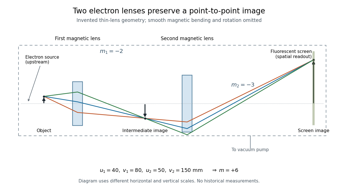
To measure magnification, divide a screen interval between corresponding grid features by the independently known object interval. Repeat over several periods to reduce endpoint uncertainty. For a proposed check, record accelerating voltage, lens electric currents, screen position and specimen orientation; compare one-stage and two-stage images, refocusing as necessary. Changing a lens electric current should change focus and scale, while a blank exposure checks detector background. Keep irradiation and recording enlargement controlled, and repeat the original setting to test drift or specimen damage. These are suggested checks, not a claim that every check was performed in 1931. A grid-scale measurement establishes magnification; resolving much finer features requires a separate target and contrast criterion.

rounding an unclipped voltage to equally spaced levels of separation $\Delta$ leaves error in $[-\Delta /2,\Delta /2]$. If the fractional position within a conversion interval is uniformly distributed, direct integration gives zero mean and expectation value $⟨{ϵ}^2⟩={\Delta }^2/12$. This is a statistical model for the error, not a claim that the converter adds independent white noise for every possible input.

A voltage is a scalar potential on the vertices of an electrical network. Away from prescribed boundary vertices it is harmonic, and its difference across an edge drives current through that edge.

A channel supporting ballistic electron transport carries incident populations set by different source and drain chemical potentials, rather than an everywhere-equilibrated local distribution with an Ohmic voltage gradient. Its electrostatic barrier responds self-consistently to contacts, gates and electrostatic screening. A symmetric rigid-barrier model places reservoir energies at $E_F\pm eV/2$ relative to the barrier. Asymmetric partition or bias-dependent transmission changes the weights in the differential electrical conductance, and must be included when extracting an energy scale.

For a finite undirected graph without self-loops, give each edge a symmetric nonnegative weight $w_{ij}=w_{ji}$. In the weighted graph, set $(A_w{)}_{ij}=w_{ij}$ for an edge and zero otherwise, and $(D_w{)}_{ii}={\sum }_j{w}_{ij}$ with all other entries zero. The Weighted graph Laplacian isEach edge appears once in the quadratic form. For the path graph $A-B-C$ with weights $w_{AB}=2$ and $w_{BC}=3$,The Weighted graph Laplacian is still a positive semidefinite matrix. Its kernel consists of vectors constant on each connected component of a graph after zero-weight edges are removed: an edge of weight zero imposes no constraint. In an electrical network, taking the weights to be electrical conductances makes $x^T{L}_{w}x$ the total power dissipated by Joule heating when $x$ gives the voltages at the vertices. This physical interpretation explains why stronger connections penalize disagreement more heavily.^[ref]

An X-ray tube accelerates electrons from a negative cathode to a positive target anode. A heated cathode supplies electrons by thermionic emission; the evacuated envelope limits collisions before the target. This differs from the gas-discharge tube in the Röntgen X-ray discovery experiment.^[ref]

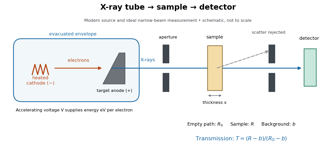
In bremsstrahlung, an electron changes velocity in the target's electric fields, emitting a photon while losing kinetic energy. Different encounters allow a continuous range of transferred energies. This is distinct from the discrete electronic transitions producing Characteristic X-rays.

Changing the accelerating voltage changes the available kinetic energy per electron and the X-ray tube cutoff. Changing the number of arriving electrons changes the number of opportunities for photon emission. These are distinct controls: a larger electric current does not by itself give each electron more energy. For an original idealized budget, $V=50\mathrm{kV}$ and tube electric current $i=0.20\mathrm{mA}$ give electrical power $Vi=10\mathrm{W}$ and arrival rate $i/e\simeq 1.25\times 10^{15}{\mathrm{s}}^{-1}$, where $e$ is the elementary charge. This is input power, not emitted X-ray power; obtaining the latter requires a conversion efficiency.

For an electron starting with negligible kinetic energy and accelerated through a constant positive electric potential difference $V$, electrical work supplies $K=eV$. In the ideal single-electron bremsstrahlung model, conservation of energy bounds any one emitted photon:The endpoint corresponds to essentially all available kinetic energy going into one photon. It is a limiting bound, not a claim that every electron produces an endpoint photon. Neglect target recoil, initial kinetic energy, and losses before the emitting interaction. If the accelerating voltage varies, its largest value sets the corresponding ideal upper endpoint; a mean voltage does not substitute for that value.

For a calculated constant-$V$ example, $50\mathrm{kV}$ gives $E_{\max }=50\mathrm{keV}$ and ${\lambda }_{\min }=0.0248\mathrm{nm}$. Doubling $V$ halves ${\lambda }_{\min }$. Producing a $0.0200\mathrm{nm}$ photon requires at least $V=hc/(e\lambda )\simeq 62.0\mathrm{kV}$ in this model. A continuous frequency spectrum spans lower photon energies; the cutoff calculation predicts neither its shape nor the efficiency of photon emission.